MPFAN: A Novel Multiscale Network for Brain Tumor MRI Classification
Authors Info & Affiliations
Abstract
Introduction
Accurate classification of brain tumours using MRI scans is vital for early diagnosis and treatment. However, conventional deep learning models often require complete MRI sequences, which can prolong scan times and lead to patient discomfort or motion-related image degradation. Thus, enhancing diagnostic accuracy under faster scanning conditions is a critical research need. Therefore, this research aims to show how our proposed mechanism, namely Multiscale Parallel Feature Aggregation Network (MPFAN), accurately improves the diagnosis of classifying brain tumours while maintaining Magnetic Resonance Imaging (MRI) quality in fast MRI scanning.
Methods
This article proposed an MPFAN architecture that utilizes parallel branches to extract image features from different scales, using independent pathways with varied filters and movement steps. Feature combination blocks, feedback prevention mechanisms, and strict training constraints enhance system reliability.
Results
MPFAN achieved an accuracy of 97.4%, outperforming many existing brain tumour classification models. Performance improved steadily over training epochs, and optimizer comparisons showed Adam and Ada-Delta yielded the best results. Ablation studies confirmed that multiscale feature extraction, dropout regularization, and feature fusion significantly contribute to classification accuracy.
Discussion
The MPFAN model demonstrates superior performance due to its ability to effectively extract and integrate multiscale features. Its dual-branch architecture enables deeper contextual understanding, and its high accuracy validates its clinical potential. However, the model’s reliance on a single dataset and potential overfitting in later training epochs indicate the need for broader validation and optimization in real-world clinical environments.
Conclusion
The proposed MPFAN architecture enhances brain tumour classification by improving image processing efficiency and decision-making speed, making it a reliable and effective diagnostic tool.
1. INTRODUCTION
Brain tumours are extremely dangerous and fatal cancers, which cause loss of life. Ageing or damaged brain cells that fail to regenerate properly may create extra tissue, leading to tumour formation [1]. Brain tumours exist in two forms: cancerous growths that spread and non-cancerous growths that do not. Fast detection and treatment of malignant brain tumours have become essential since they spread rapidly into nearby brain tissues to increase the chances of survival [2].
Doctors often choose MRI scans to discover brain tumours because these devices create precise brain images through magnets instead of radiation exposure. Brain tumours are generally categorized into three types based on their location: meningiomas, pituitary tumours, and gliomas [3]. There are two main brain tumour image classification strategies using MRI scans: traditional manual feature analysis and deep learning techniques. Doctors must select image features by hand before feeding them into standard classifiers, including Support Vector Machine (SVM) and K-Nearest Neighbour (KNN). These methods work well but take a long time to process data and require a lot of effort [4-7]. Convolutional Neural Networks (CNNs) enable deep learning systems to automatically identify and organize features while addressing challenges related to improper data and slow processing.
Standard deep learning approaches need all the information within the MRI images to perform classification. Extended MRI procedures make patients uncomfortable and result in damaged MRI images when patients move. Deep learning methods for fast MRI scanning must improve their ability to preserve image quality to achieve better brain tumour classification results [8, 9].
Our proposed MPFAN architecture combines CNN features from different scales through parallel networks to boost brain tumour classification results. MPFAN uses parallel branches to extract detailed image features both near and far. The system uses two independent pathways to examine input images using different filters and movement steps to produce different feature sets. Integrating separate feature combination blocks, feedback prevention tools, and strict training limits helps the system perform more reliably. The proposed method combines efficient brain tumour classification with powerful diagnostic results through better processing and quicker decision-making. The main contribution of the paper is as follows:
- We present a state-of-the-art method to classify brain tumours from MRI images.
- We present a Multiscale Parallel Feature Aggregation Network (MPFAN) to detect tumours efficiently from medical images.
- We experimentally explore this network for different parameters.
1.1. Related Work
The current literature on glioma grading and brain tumour classification predominantly relies on CNN-based methods due to their ability to learn local features. However, these methods struggle with modelling long-range dependencies and global context, which may limit classification accuracy. The machine learning-based approach discussed by Wang et al. demonstrates satisfactory accuracy but provides limited insights into general performance across various tumour classes [10].
Attention mechanisms have increased the emphasis on features, yet convolutional operations still dominate, making capturing objects such as blurred edges or intensity variations challenging. On the other hand, previous approaches achieve high accuracy; further enhancements are needed to develop more general and multiscale classifiers. Rasheed et al. employed an efficient CNN method to categorize three different types of brain tumors [11]. Abd El-Wahab et al. proposed a deep learning model called BTC-FCNN to enhance classification accuracy while reducing the computational overhead of MRI-based classifiers [12].
Ozkaraca et al. utilized Dense CNN to improve brain tumour classification in MRI imaging [13]. Similarly, Muezzinoglu and Others introduced PatchResNet, a framework leveraging multi-sized patch-based feature fusion to achieve high classification accuracy [14]. Their approach incorporates KNN classification and iterative hard voting, which are crucial for boosting accuracy. Mijwil et al. employed MobileNetV1 to classify brain tumors in MRI images, demonstrating an accurate and efficient model for medical imaging systems [15]. Saurav et al. introduced a simple attention-guided convolutional neural network (AG-CNN) architecture that utilizes channel attention and global average pooling (GAP) as its feature extraction mechanism [16].
Sekhar et al. adopted the GoogLeNet model and employed SVM and KNN classifiers to differentiate gliomas, meningiomas, and pituitary tumors [4]. Athisayamani et al. utilized ResNet152 to enhance feature extraction and reduce dimensionality, improving classification performance [17]. Shahin et al. designed MBTFCN, which classifies tumors across multiple categories using three key techniques, including feature extraction with residual connections and attention mechanisms [18].
In their research, Aloraini et al. integrated Transformer and CNN elements into a single model, while Zulfiqar et al. leveraged EfficientNets for brain tumor image classification [19, 20]. Mehnatkesh et al. [21] applied an improved ant colony algorithm to optimize MRI tumor classification using ResNet. Singh and Agarwal developed a CNN-based approach specifically designed for T1WCE MRI images [22].
Isunuri and Kakarla utilized a neural network based on separable convolution to maximize computational speed in tumor classification [23]. Raza et al. extended GoogLeNet into a 15-layer deep network to enhance expressive capabilities [24]. Aamir et al. employed EfficientNet-B0 for feature extraction after grouping and segmenting images, enhancing image contrast using nonlinear techniques [25].
A new approach, referred to as full-stack learning (FSL), was proposed by Wang et al., where sampling, reconstruction, and segmentation are co-performed due to task dependencies and improve MRI workflow [26]. Ling et al. proposed a new multitask attention network named MTANet for better segmentation and classification, together with an attention mechanism [27]. Wang et al. developed a multi-stage hybrid attention network (MHAN) model to conduct MRI image super-resolution and reconstruction, besides having specialized modules regarding enhanced spatial feature extraction [28]. Sui et al. applied ConvNext blocks in a multi-task learning system for liver MRI analysis and found refined details for higher accuracy [29]. Subsequently, Delannoy et al. proposed SegSRGAN, which employs the GANs to improve the resolution in neonatal brain MRI and the segmentation accuracy [30]. Corona et al. integrated total variation reconstruction and Chan-Vesed segmentation using nonconvex Bregman iteration to achieve enhanced output from both systems [31]. Cipolla et al. also presented a structure that uses geometric and semantic loss to allow scene analysis with maximum efficiency in multi-task learning [32]. Sun et al. developed SegNetMRI as a deep learning technology that reconstructs and segments MRI images using compressed sensing techniques [33]. Sui et al. developed RecSeg to incorporate two U-Net structures, making MRI reconstruction faster and lesion segmentation more accurate [34]. Pramanik and Jacob recently employed Deep-SLR to improve the parallel MRI data reconstruction and segmentation function [35].
Recent studies also highlight the use of Electroencephalogram (EEG)-based machine learning models and their application to different neurological disorders with an unmatched accuracy rate [36]. Tripathi et al. developed a Weka-based ensemble framework that integrated EEG, Electrocardiogram (ECG), and Electromyography (EMG) signals working with the PhysioNet sleep-bruxism dataset [37]. They reported up to 99% accuracy in detecting sleep bruxism. M.B. Bin Heyat et al. [38], which used a Decision Tree classifier with C4–P4 and C4–A1 EEG channels for sleep bruxism detection [39-41]. Wang et al. proved that single-channel EEG (C4–P4) and some fine decision tree classifiers could achieve 97.84% accuracy using a small REM-sleep dataset for bruxism detection [42]. In the Attention Deficit Hyperactivity Disorder (ADHD) diagnosis, Saini et al. suggested a model to predict ADHD using EEG signals and machine learning methods [43]. This method tested different types of classifiers to improve the accuracy and reliability of the diagnosis of ADHD. The proposed method showed how EEG-based automated systems can help in early identification and can be useful for clinical use. Regarding epilepsy detection, Alalaya et al. suggested a method to detect epilepsy using EEG signals [44]. This method used DWT to extract features and then used PCA or t-SNE to reduce the complexity of the data. Several classifiers, such as RF, XGBoost, and MLP, were tested to see which one works best. This method achieved an accuracy of up to 98.98%, which is better than the accuracy reported in previous research.
Table 1 presents a comparative analysis of various deep learning models (CNNs, CNNs with Attention, and Transformers) for classifying Computed Tomography (CT) scans as belonging to a brain tumour [45-50]. It proved that CNNs can be more accurate when used, but they have a variety of limitations, such as capturing the global context or the long-range dependencies. The incorporation of attention-based models enhances feature focus but, at the same time, presents problems such as blurred boundaries and marginal classification errors. Thus, although transformer models seem to be accurate in many tasks, limited data exists comparing them to other techniques for glioma grading or multi-class categorization.
| Author(s) | Methodology | Key Features | Strengths | Remarks |
|---|---|---|---|---|
| Rasheed et al. [11] | CNN | Three-class classification | Efficient feature learning | Baseline CNN; lacks advanced context handling |
| Abd El-Wahab et al. [12] | BTC-FCNN | Fast CNN for MRI | High accuracy, low computation | Prioritizes speed; suited for real-time systems |
| Ozkaraca et al. [13] | Dense CNN | Dense connections | Enhanced feature propagation | Strong feature reuse, but risk of redundancy |
| Muezzinoglu et al. [14] | PatchResNet + KNN | Patch-based deep fusion | Multi-size patch learning | Creative patchwise fusion with classical ML |
| Mijwil et al. [15] | MobileNetV1 | Lightweight CNN | Efficient, mobile-friendly | Suitable for edge deployment |
| Saurav et al. [16] | AG-CNN | Attention + GAP | Emphasizes relevant features | Emphasizes spatial attention for classification |
| Sekhar et al. [4] | GoogLeNet + SVM/KNN | Hybrid deep + classical ML | Effective multi-class separation | Combines deep and traditional techniques |
| Athisayamani et al. [17] | ResNet152 | Feature extraction + reduction | Strong residual learning | Deep architecture with reduced overfitting |
| Shahin et al. [18] | MBTFCN | Residual + attention | Modular, scalable design | Modular framework with strong potential |
| Aloraini et al. [19] | Transformer + CNN | Hybrid deep learning | Captures long-range dependencies | Innovative mix of CNN and Transformer |
| Zulfiqar et al. [20] | EfficientNet | Efficient CNN model | High accuracy, low parameters | Balanced accuracy and efficiency |
| Mehnatkesh et al. [21] | ResNet + Ant Colony Optimization | Feature optimization | Intelligent hyperparameter tuning | Uses bio-inspired tuning; novel combo |
| Singh & Agarwal [22] | CNN for T1WCE | Tailored to specific MRI type | Better domain-specific accuracy | Specialized approach for T1WCE modality |
| Isunuri & Kakarla [23] | Separable Conv Net | Faster computation | Optimized inference speed | Prioritizes speed with separable convolutions |
| Raza et al. [24] | Deep GoogLeNet (15-layer) | Extended depth | Richer feature extraction | Deep stack model for richer features |
| Aamir et al. [25] | EfficientNet-B0 + Image Segmentation | Contrast enhancement + segmentation | High classification precision | Strong results with preprocessing boost |
| Wang et al. [26] | Full-stack AI | Joint sampling, segmentation | Streamlined MRI workflow | Holistic pipeline from input to diagnosis |
| Ling et al. [27] | MTANet | Multi-task with attention | Strong joint segmentation & classification | Multi-task enhances robustness |
| Wang et al. [28] | MHAN | Multi-stage hybrid attention | Effective feature refinement | Layered attention improves accuracy |
| Sui et al. [29] | ConvNext + multi-task | MRI liver analysis | High accuracy in multi-task setting | Great potential, but for liver MRI |
| Delannoy et al. [30] | SegSRGAN | GAN for segmentation + SR | High-resolution segmentation | Combines SR with accurate segmentation |
| Corona et al. [31] | Nonconvex Bregman Iteration | Joint reconstruction + segmentation | Strong theoretical foundation | Mathematical rigor, practical challenge |
| Cipolla et al. [32] | Multi-task + uncertainty loss | Loss weighting via uncertainty | Efficient scene understanding | Smart uncertainty-based multitasking |
| Sun et al. [33] | SegNetMRI | Unified DL for MRI | Effective joint learning | Specific to compressed sensing |
| Sui et al. [34] | RecSeg (dual U-Net) | Fast MRI + lesion segmentation | Robust to noise, high accuracy | Redundant dual net improves segmentation |
| Pramanik & Jacob [35] | Deep-SLR | Image domain deep learning | Better parallel MRI handling | Deep learning for fast, quality MRI |
| Tripathi et al. [37] | Ensemble learning using Weka with EEG, ECG, EMG fusion | Power spectral density (EEG), multi-signal fusion, PhysioNet dataset | strong multi-modal approach | Combining EEG with ECG/EMG greatly enhances bruxism detection accuracy |
| Wang et al. [42] | Fine decision tree classifier on single-channel EEG | Time-frequency, nonlinear features, bipolar channels (e.g., C4–P4) | simplicity of single-channel use | Single EEG channel (C4–P4) sufficient for accurate bruxism classification |
| Saini et al. [43] | Applied Naïve Bayes, K-NN, and Logistic Regression on EEG dataset for ADHD prediction | Dataset of 157 children (77 ADHD, 80 healthy), behavioral symptom analysis | K-NN achieved highest accuracy (89%), better than Naïve Bayes and Logistic Regression | Useful for ADHD diagnosis in children |
| Alalayah et al. [44] | DWT for feature extraction, PCA and t-SNE for dimensionality reduction, classifiers: RF, XGBoost, K-NN, DT, MLP | EEG signals, DWT features, PCA + t-SNE, K-means clustering | Achieved 98.98% accuracy using MLP with PCA + K-means, high precision and F1-score | Effective for early epilepsy detection |
2. PROPOSED METHODOLOGY
Fig. (1) shows the method to classify brain tumours using Magnetic Resonance Imaging scans. Before analysis begins, researchers resize images and eliminate noise by applying a Wiener filter followed by a smoothing process. The Wiener filter enhances image quality by responding to local variations and fighting noise to keep vital edge and texture information that doctors need to diagnose correctly. We normalize and prepare input data before deep learning models perform their processing tasks.
The pre-processed images enter the MPFAN model to dig out functional image content. MPFAN uses multiple processing pathways to examine different kinds of image features at various levels of detail, while attention techniques highlight the most important image areas. The model classifies the images into four categories: The system reacts to MR image input by labelling results into four tumour groups, which include “No Tumour,” “Glioma,” “Pituitary,” and “Meningioma.” The system combines improved processing steps with MPFAN’s focused analysis to help doctors make accurate tumour-type detections.
2.1. Image Preprocessing
Using Wiener filtering enhances medical images accurately, especially when performing vital tasks in medical imaging research [51]. This method lowers image noise to boost overall quality without harming distinct structural and textural parts. Wiener filtering helps prepare MRI images for brain tumour classification before deep learning models can analyze them. The Wiener filter adjusts to image areas to find noise power and then applies ideal smoothing to each region. Compared to standard filters, the Wiener filter keeps vital medical image information intact. It does so by considering both the signal-to-noise ratio and the local variance within the image (Eq. 1), reducing noise selectively without compromising sharpness.
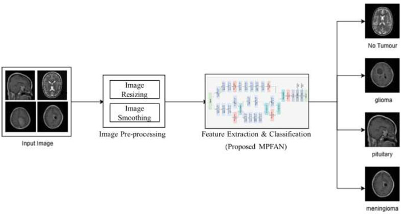
Workflow of the proposed MPFAN-based brain tumour classification
 |
(1) |
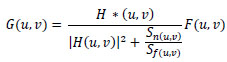
Where G(u,v) is the restored image, H(u,v) represents degradation functions, and F(u,v) is a degraded image in the frequency domain. Here, the power spectral density is represented by Sn(u,v) and Sf(u,v) for noise and the original image, respectively.
Processing MRI images initially helps remove acquisition noise and environmental interference that may interfere with tumour observation. Wiener filtering both boosts visual contrast and corrects distorted input data to make the results clearer and of better quality. Our deep learning model achieves better detection precision by operating on images that retain natural structure and shape details. The processing system can accurately recognize brain tumours through MRI scans thanks to the Wiener filtering application.
2.2. Proposed Algorithm: Multiscale Parallel Feature Aggregation Network (MPFAN)
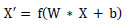
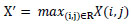
A multi-branch convolutional neural network (CNN) architecture incorporating a multiscale feature extraction architecture is proposed to learn multiscale features effectively and achieve robust performance, as shown in Fig. (2). It has an input layer of image shape 120 × 120 × 3. The input is processed independently in two parallel branches using convolutional layers (conv1 and conv2) with different kernel sizes and strides. By this configuration, the network can extract different features of the input images. Eqs. 2 and 3) represent the convolution and max pooling operations that are applied to the images.
 |
(2) |
 |
(3) |
Where W, X, and b are kernel, input, and bias, respectively, followed by activation function f(.).
Each branch consists of a series of convolutional blocks, which are then finished with maxpooling layers to decrease spatial measurements while keeping significant hierarchical information. One of the key features of the architecture is the use of concatenation layers, which combine feature maps of different branches. The same is shown in Eq. (4), which allows the network to retain and integrate information from multiple scales, preserving global and local spatial patterns.
 |
(4) |
To take advantage of the higher accuracy of Thompson sampling on stochastic bandit problems, we propose a multi-branch approach that allows for more complex input data by combining empirical value estimates with Thompson sampling. After the feature extraction process, the network transitions to fully connected layers for high-dimensional transformation and classification. The first step is to flatten the feature maps, transforming the 3D tensors into 1D feature vectors.
Architecture of the proposed Multiscale Parallel Feature Aggregation Network (MPFAN).
In the first dense layer, we set the number of neurons to 2048 to learn complex patterns (beyond simple lines and planes) in the data. These learned features are passed through a second dense layer with 512 neurons for further refinement. To prevent the model from overfitting, dropout layers with well-chosen rates are applied after each dense layer to ensure that the model generalizes well to unseen data. Depending on whether the task is binary classification, the final dense layer consists of a single neuron with either a linear or sigmoid activation function. Eq. (5) shows the functionality of a fully connected layer, and softmax classification is represented by Eq. (6).
 |
(5) |
 |
(6) |
With its multi-branch design, layered structure, feature concatenation, and regularization techniques, the network is naturally suited for tasks that require high-dimensional input processing and precise feature extraction and classification.
2.3. Pseudo Code for MPFAN
Our MPFAN model implementation starts by defining the size of the MRI image inputs. The input layer processes the images and passes them through two separate convolutional branches: one with a smaller filter size. Our design uses one convolutional branch with 3 × 3 filters and another with 5 × 5 filters. These layers shrink feature maps by taking their maximum values during each subsampling step. The model merges scale feature maps from each input branch to build its overall representation.
A layer of 2048 neurons with ReLU activation builds complex features that reduce the dropout layer with 0.4 probability to prevent overfitting. After processing through 512 neurons, the layer refines another step-in feature extraction before traditional dropout protection. The model’s final layer consists of one neuron with a sigmoid activation to provide tumour malignancy likelihood. The model trains best using Adam optimization and binary cross-entropy loss to achieve proper results. The same has been presented as an algorithm in Algorithm 1 for the proposed MPFAN model.
Algorithm 1: Multiscale Parallel Feature Aggregation Network (MPFAN)
1: Input: MRI brain image I∈R120×120×3
2: Output: Tumour classification y∈{Glioma,Meningioma,Pituitary,No Tumour}
3: Load MRI brain tumour image of size 120 × 120 × 3.
4: FA1 ← ReLU(Conv2D32,3×3,s=2(I))
5: FA2 ← ReLU(Conv2D32,3×3,s=1(FA1))
6: FA3 ← ReLU(Conv2D64,3×3,s=1(FA2))
7: PA ← MaxPool3×3(FA3)
8: PA” ← ReLU(Conv2D64,3×3,s=2(FA3))
9: Concatenate: F1 ← Concat(PA, PA”)
10: FC1 ← ReLU(Conv2D64,1×1,s=1(F1))
11: FC2 ← ReLU(Conv2D64,5×1,s=1(FC1))
12: FC3 ← ReLU(Conv2D64,1×5,s=1(FC2))
13: FC4 ← ReLU(Conv2D96,3×3,s=1(FC3))
14: FD1 ← ReLU(Conv2D64,3×3,s=1(F1))
15: FD2 ← ReLU(Conv2D96,5×5,s=1(FD1))
16: Concatenate: F2 ← Concat(FC4, FD2)
17: PF2 ← MaxPool3×3(F2)
18: FE1 ← ReLU(Conv2D96,3×3,s=1(F2))
19: Concatenate: F3 ← Concat(PF2, FE1)
20: FB1 ← ReLU(Conv2D64,1×1,s=2(I))
21: FB2 ← ReLU(Conv2D64,3×1,s=1(FB1))
22: FB3 ← ReLU(Conv2D64,1×3,s=1(FB2))
23: PFB3 ← MaxPool3×3(FB3)
24: FE1 ← ReLU(Conv2D64,1×1,s=1(PFB3 ))
25: FE2 ← ReLU(Conv2D64,5×1,s=1(FE1))
26: FE3 ← ReLU(Conv2D96,1×5,s=1(FE2))
27: FE4 ← ReLU(Conv2D96,1×1,s=2×1(FE3))
28: FE5 ← ReLU(Conv2D96,3×3,s=1(FE4))
29: PFE5 ← MaxPool3×3(FE5)
30: Concatenate: F4 ← Concat(PFE5, F3)
31: P3 ← MaxPool3×3(F4)
32: Flatten the pooled feature map: Ff ← Flatten(P3)
33: Fully connected layer 1: h1 ← ReLU(W1Ff + b1), then apply Dropout (p = 0.4)
34: Fully connected layer 2: h2 ← ReLU(W2h1 + b2), then apply Dropout (p = 0.4)
35: Final output: yˆ← Softmax(W3h2+ b3)
36: Predicted class: y ← Argmax(yˆ)
The algorithm is run on an MRI dataset with 32 images per batch during 100 training rounds. We use labeled MRI images to train our model and validate performance by checking results with the validation data. The MPFAN model achieves good results while also running efficiently for brain tumour diagnosis tasks.
2.4. Dataset Description
The Brain Tumour MRI Dataset provides a comprehensive collection of MRI scans for brain tumour classification [52, 53]. It includes four tumour categories: Gliomas (300 images), Meningiomas (306 images), Pituitary Tumours (300 images), and No Tumours (405 images). This dataset is well-suited for deep learning applications focused on automatic tumour detection and classification.
| Epoch | TA | TL | TP | TR | TF | VA | VL | VP | VR | VF |
|---|---|---|---|---|---|---|---|---|---|---|
| 20 | 0.956 | 0.092 | 0.958 | 0.956 | 0.951 | 0.961 | 0.082 | 0.962 | 0.961 | 0.957 |
| 40 | 0.975 | 0.069 | 0.976 | 0.974 | 0.971 | 0.975 | 0.064 | 0.975 | 0.975 | 0.973 |
| 60 | 0.983 | 0.055 | 0.983 | 0.982 | 0.98 | 0.986 | 0.057 | 0.987 | 0.984 | 0.98 |
| 80 | 0.984 | 0.055 | 0.985 | 0.984 | 0.983 | 0.964 | 0.078 | 0.966 | 0.964 | 0.958 |
| 100 | 0.985 | 0.053 | 0.985 | 0.985 | 0.983 | 0.974 | 0.072 | 0.977 | 0.974 | 0.974 |
R=Recall, F=F1-Measure.
| Optimizer | TA | TL | TP | TR | TF | VA | VL | VP | VR | VF |
|---|---|---|---|---|---|---|---|---|---|---|
| RMS Prop | 0.922 | 0.129 | 0.93 | 0.919 | 0.918 | 0.887 | 0.195 | 0.894 | 0.878 | 0.869 |
| Ada-Delta | 0.99 | 0.042 | 0.991 | 0.99 | 0.989 | 0.972 | 0.071 | 0.977 | 0.972 | 0.97 |
| Adam | 0.985 | 0.053 | 0.985 | 0.985 | 0.983 | 0.974 | 0.072 | 0.977 | 0.974 | 0.974 |
| SGD | 0.987 | 0.05 | 0.988 | 0.987 | 0.986 | 0.958 | 0.113 | 0.959 | 0.958 | 0.953 |
| AdaGrad | 0.98 | 0.058 | 0.98 | 0.979 | 0.975 | 0.964 | 0.078 | 0.966 | 0.963 | 0.96 |
Given the challenges of low-quality imaging and undersampled data, our MPFAN model addresses these issues by extracting multiscale features and processing them in parallel. The dataset is used for both training and performance evaluation of the MPFAN model, with key aspects including multiscale feature extraction to capture tumour characteristics at different spatial levels, parallel processing for improved feature representation, and classification accuracy, efficiency, and feature robustness as the primary performance metrics.
3. RESULTS AND DISCUSSION
The comparative analysis of different epochs indicates a consistent improvement in performance metrics over time, as shown in Table 2. Validation and training accuracy increase as the model trains from 20 to 100 epochs. At epoch 100, the validation accuracy hits 0.974 while training accuracy reaches 0.985. As the model trains over time, its optimization improves, resulting in lower training (0.053) and validation loss (0.072). The changes in TR and TF results ensure better model performance, while TP gains show steady progress in reliability. Our results show signs of overfitting from validation metrics in later epoch updates. Our findings show that increasing model training time produces better results yet requires manual optimization to maintain prediction reliability.
The analysis finds that Ada-Delta is the most effective optimizer because it delivers top accuracy (0.990) and validation accuracy (0.972) across all performance measures. In Table 3, Adam’s superior performance shows that this optimizer produces 0.985 top accuracy and 0.974 validation accuracy. Gradient Descent proves itself through a Test Accuracy (0.987) that is slightly lower than its Validation Accuracy (0.958). In performance testing, AdaGrad generates acceptable results with accuracy scores of 0.980 for training and 0.964 for validation. RMS Prop ranks lowest among tested optimizers because it achieves a TA of 0.922 and a VA of 0.887 compared to other optimization methods.
As illustrated in Fig. (3), the trade-off curves capturing the model's learning dynamics on brain tumor classification showcase the trade-offs between accuracy, loss, precision, recall, and F1-score. Inaccuracy measurement subsection (Fig. 3a), training accuracy appears to improve throughout epochs and levels off at around 98.5% while validation accuracy plateaus slightly below at about 97.4%. This indicates strong model generalization with negligible overfitting issues. Validation loss presented in slice (Fig. 3b) demonstrates trends linking cross-entropy losses for both datasets, whereby training loss decreases to a value of 0.053 and validation loss settles just under 0.072, confirming effective convergence without underfitting issues persisting. These observations support claims regarding high optimisation efficiency provided by applying the Adam algorithm, as well as confirming that the model acquires proper representations during the training phase, unexposed to excessive overfitting or underfitting during alternating training and validating stages.
The model's classification performance is further analyzed and highlighted in training and validation using precision, recall, and F1-score curves shown in subfigures (Fig. 3c-e). The training precision peaks at 98.5% while validation precision stabilizes around 97.7%, reinforcing the claim that false positives are minimized. Also, recall values, which indicate a model's sensitivity, hit 98.5% for training and 97.4% for validation, which means almost all true tumor cases are captured. The F1-score captures both precision and recall, achieving 98.3% on the training set while validation yields 97.4%. Having strong results across the board reflects the classification ability of the model.
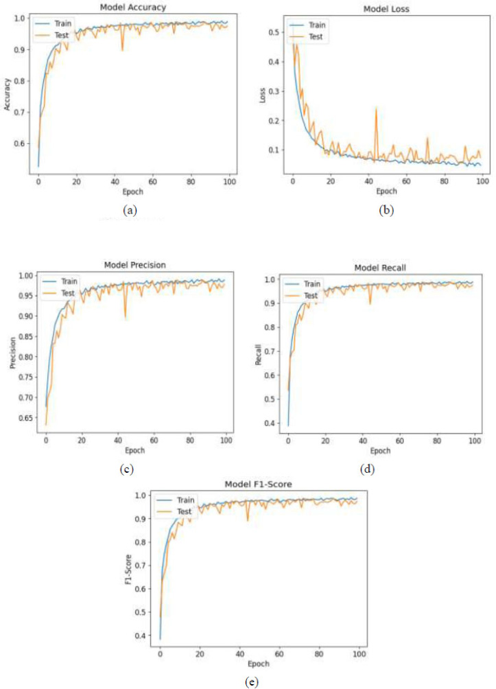
Trade-off curves between training and validation (a) Accuracies, (b) Loss, (c) Precision, (d) Recall, (e) F1-Score
Comparison with Existing Methods.
The close distance of these metrics across training and validation illustrates the strength of the model, alongside its stability over epochs, suggesting strong overall performance even with multilabel medical images from diverse domains within healthcare fields spanning many specialties. All together, these confirm that the accuracy estimations reached by the proposed model for real-time detection of brain tumors in support systems are trustworthy.
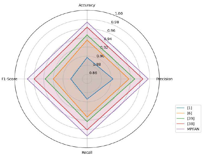
3.1. Comparison with Existing State-of-the-Art
This study compares MPFAN against leading brain tumour classification techniques that exist today, as found in Fig. (4). The MPFAN system delivers outstanding performance in every metric, with a precision of 0.977 and outcomes that closely match each other. MPFAN performs better than competing systems, which reported 0.963 accuracy and 0.960 F1 measure data. Our study shows that breaking up tumour features at multiple scales and then analyzing them together improves detection accuracy to establish a new classification benchmark.
3.2. Ablation Study
We have performed an extensive ablation study to understand the contribution of each architectural component of the proposed MPFAN model. Here, we have tested the performance impact of removing or modifying important components such as the multi-branch structure, feature fusion strategy, dropout regularization, optimizer, and dense layer configuration. Table 4 presents the results of the comparative analysis of each architectural component of MPFAN. The baseline MPFAN model achieved a classification accuracy of 97.4% on the brain tumor MRI dataset. Removing one of the parallel branches (3×3 or 5×5 convolution) caused a drop in accuracy to 93.1%, underscoring the importance of extracting multiscale features. Additionally, using the same kernel size in both branches, accuracy dropped to 94.5%, suggesting that capturing rich spatial features requires multiple receptive fields.
| Description | Accuracy (%) | Drop in Accuracy w.r.t. MPFAN |
|---|---|---|
| Proposed Method (MPFAN) | 97.4 | - |
| Remove one parallel branch (use only 3×3 conv) | 93.1 | ↓ 4.3 |
| Use same kernel size in both branches (3×3 for both) | 94.5 | ↓ 2.9 |
| Remove feature concatenation (keep outputs separate) | 91.8 | ↓ 5.6 |
| Remove dropout layers | 95.2 | ↓ 2.2 |
| Reduce dense layer size (1024 → 256 instead of 2048 → 512) | 94.7 | ↓ 2.7 |
| Replace Adam with SGD optimizer | 95.8 | ↓ 1.6 |
| Remove max pooling in branches | 92.5 | ↓ 4.9 |
| Single-scale CNN (no multiscale branches) | 90.4 | ↓ 7.0 |
Moreover, eliminating the concatenation of features also resulted in a notable accuracy drop to 91.8%, underscoring its vital role in maintaining multiscale spatial quantitative information. The removal of dropout also reduced accuracy to 95.2%, confirming the regularization effect of dropout, which is clearly necessary in avoiding overfitting.
The accuracy is dropped to 2% (i.e., 94.7%) with the modification changing dense layers from 2048→512 to 1024→256. This shows a need for greater feature transformation ability in the classification phase. Changing the optimizer from Adam to SGD caused a slight drop to 95.8%, suggesting better convergence properties of Adam for this architecture. Also, removing max pooling in the branches or using a single-scale CNN (no multi-branch structure) caused a significant loss in performance, down to 92.5% and 90.4%, respectively. These results support the design choices made in the MPFAN and illustrate the need for multiscale processing in parallel with hierarchical feature integration to achieve precise brain tumor classification.
3.3. Constraints of the Study
Results aside from the strong performance of the proposed MPFAN model in brain tumor classification, MPFAN shows several limitations that may most likely impact interpretation and generalization. The model is trained and validated using a single benchmark MRI dataset, which does not consider the variability present in real-world clinical scenarios with different imaging devices, patient demographics, and scanning protocols.
Moreover, the model demonstrated high accuracy across epochs and optimizers; however, signs of overfitting at the later stages of training indicate that there could be a sensitivity to performance related to the training duration and the hyperparameter settings. Furthermore, the fixed choices of parameters, like the optimizer and the architectural designs used, may pose barriers to reproducibility and scalability without some form of automated optimization. Although the ablation study validated that every architecture component is important, the study did not address the robustness of MPFAN under noise in the data or incomplete information, which tend to be more prevalent in clinical settings. Such shortcomings need to be addressed in subsequent work to improve the model’s clinical relevance and potential for widespread use.
4. CONCLUSION AND FUTURE DIRECTIONS
The MPFAN (Multiscale Parallel Feature Aggregation Network) model is developed to improve brain tumor detection by parallel feature extraction at multiple scales. MPFAN can capture fine-grained local and global contextual patterns in MRI brain scans with its multi-branch convolutional architecture and hierarchically integrated feature fusion approach. MPFAN overcomes challenges like feature redundancy, insufficient multiscale pattern representation, and poor computation efficiency in traditional CNN models by concurrently processing image data from varying receptive fields, effectively integrating them. This marks a stark difference from our model, which, while still being resource considerate, enables low-resource demand environments like clinical settings to leverage the model in real-time.
As for work to tackle in the future, we intend to optimize MPFAN by adding an Attention Fusion Network to supersede conventional concatenation layers. This will allow the network to selectively concentrate on the most important feature maps during training and inference processes, making the model achieve these tasks much faster, reducing overfitting, and lowering model complexity. Moreover, we plan to add residual connections and bottleneck structures to strengthen the gradient flow and improve convergence and generalization performance. For future research, we want to modify the architecture of MPFAN for use in multimodal medical imaging, like combining MRI with PET or CT scans, while also broadening its use to include the classification of various neurological and oncological abnormalities. Moreover, the explainability modules, such as Grad-CAM or SHAP, may be examined to enhance clinical trust and provide insight into the network's reasoning. With such enhancements, the MPFAN can develop into a strong, flexible architecture for a complete analysis of medical images.
AUTHORS’ CONTRIBUTIONS
The authors confirm their contribution to the paper as follows: M.A.A., A.M.: Conceptualization; B.D.S.: Data analysis or interpretation; S.A., P.S., M.D., S.A.: Draft manuscript. All authors reviewed the results and approved the final version of the manuscript.
LIST OF ABBREVIATIONS
| MPFAN | = Multiscale Parallel Feature Aggregation Network |
| MRI | = Magnetic resonance imaging |
| CNN | = Convolutional Neural Network |
| SVM | = Support Vector Machine |
| KNN | = K-Nearest Neighbour |
| AG-CNN | = Attention-Guided Convolutional Neural Network |
| GAP | = Global Average Pooling |
| BTC-FCNN | = Brain Tumour Classification-Fast Convolutional Neural Network |
| MBTFCN | = Modular Brain Tumour Fully Convolutional Network |
| MTANet | = Multi-task Attention Network |
| MHAN | = Multi-stage Hybrid Attention Network |
| GAN | = Generative Adversarial Network, |
| EEG | = Electroencephalogram |
| ECG | = Electrocardiogram |
| EMG | = Electromyography |
| DWT | = Discrete Wavelet Transform |
| ADHD | = Attention Deficit Hyperactivity Disorder |
| SGD | = Stochastic Gradient Descent |
| ReLU | = Rectified Linear Unit. |
AVAILABILITY OF DATA AND MATERIAL
The data supporting the findings of the article is available in the Kaggle repository at https://www.kaggle.com/datasets/masoudnickparvar/brain-tumor-mri-dataset, reference number [53].
CONFLICT OF INTEREST
Dr. Salman Akhtar is the Associate Editorial Board Member of The Open Bioinformatics Journal.
ACKNOWLEDGEMENTS
declared none.