A Dual CT Image Denoising Approach using Guided Filter and method-based Noise in the NSST Domain
Authors Info & Affiliations
Abstract
Introduction
Low-dose Computed Tomography (LDCT) images are often corrupted by Gaussian noise owing to electronic interference and environmental factors during image acquisition. This type of noise significantly degrades image quality, obscures fine structural details, and hinders accurate medical interpretation. To overcome this, the current study aims to develop an effective denoising method that suppresses Gaussian noise, preserves edges and sharp features, and improves the overall visual quality. The proposed method outperforms existing denoising techniques in terms of Peak Signal-to-Noise Ratio (PSNR), Structural Similarity Index Measure (SSIM), Entropy Difference (ED), Feature Similarity Index Measure (FSIM), and Root Mean Squared Error (RMSE), thereby improving overall diagnostic precision.
Methods
The proposed denoising method integrates the Nonsubsampled Shearlet Transform (NSST), guided filtering, and BayesShrink thresholding method in a dual-stage process. Initially, the NSST process decomposes the noisy CT image into approximation and detail components. The approximation component is improved using guided filtering to preserve fine structural details, whereas detail components are denoised using BayesShrink thresholding for noise reduction. A method noise-based approach is then evaluated and further enhanced by applying NSST and BayesShrink methods to the residual part. Finally, the denoised outputs from the two stages are fused to reconstruct the final denoised CT image. The comparative evaluation of the proposed method against Discrete Wavelet Transform (DWT), NSST with bilateral filtering, Method noise-based Convolutional Neural Network (CNN), NSST with Bayes shrinkage, NSST with Wiener filtering, and Stein’s Unbiased Risk Estimate Linear Expansion of Thresholds (SURELET), and Tetrolet transform. Quantitative evaluation metrics (PSNR, SSIM, ED, FSIM, and RMSE) were used across varying noise levels (σ = 5,10,15,20), confirming its consistent superiority in noise suppression and edge preservation.
Results
The proposed denoising method consistently outperformed all other standard methods at varying noise levels. It achieved higher PSNR and SSIM values, lower RMSE values, and enhanced ED and FSIM values. These experimental outcomes demonstrate superior denoising performance in terms of both noise reduction and edge detail preservation.
Discussion
The integration of NSST with guided filtering and Bayesian thresholding significantly improves the denoising ability in LDCT images without degrading the fine image details. The iterative method noise-based refinement process improved the denoising performance. Although computationally intensive, the proposed method is clinically applicable, specifically in lower-dose imaging scenarios.
Conclusion
This study demonstrates a hybrid denoising approach that combines NSST, BayesShrink thresholding, guided filtering, and method noise-based refinement process. The method shows remarkable efficacy in suppressing Gaussian noise while preserving edge and structural details, thereby improving diagnostic quality in low-dose CT images.
1. INTRODUCTION
CT imaging is a crucial modality in therapeutic diagnostics that helps in examining the complications related to the human body. It provides crucial information for disease diagnosis, surgical planning, and treatment monitoring [1-3]. However, CT scans use different sensors to capture CT images, making them more susceptible to noise. CT images are generated using X-ray radiation. However, exposure introduces noise and artifacts during image acquisition and transmission owing to factors such as low radiation dose, equipment constraints, and patient movement. However, while higher radiation improves imaging quality, excessive exposure poses health risks.In LDCT imaging, these issues often result in uncertainty in medical diagnosis. The most common noise types are Gaussian and Poisson noise, with Gaussian noise following a Gaussian distribution [4]. Gaussian noise often compromises the quality of low-dose images, posing a significant challenge to precise clinical diagnostics. It can obscure crucial information, making it difficult to detect lesions and recognize abnormalities. Photon shot noise, electrical signal interference, and transmission errors generate a grainy, pseudo-random texture in the image, causing distortion and the reduction of intricate information.
Image denoising is a major step for noise reduction and detail retention such as edges and textures, thereby improving its quality and clarity. Over the past few decades, researchers have developed different methods to address image-denoising issues [5]. Traditional methods include sinogram filters, iterative reconstruction methods, and post-processing methods. Sinogram-based filters initially preprocess sinogram information, then reconstruct the sinogram to a CT image using a filter back projection algorithm. A sinogram is denoted as the raw data collected from a CT scan, which represents projectional information of a specific object at various angles. The projection space methods like stationary wavelet transform, penalized weighted least squares, and sinogram smoothing suppress noise in sinograms. The main limitation of sinogram filtering methods is the potential for data inconsistency, which can lead to artifacts in reconstructed LDCT images [6-8].
Iterative reconstruction methods rely on both the sinogram and image domains to obtain high-quality CT images. Researchers have proposed multiple methods aimed at noise suppression in CT images. Unlike the traditional Filtered-Back Projection (FBP), which reconstructs the image using a single pass, iterative reconstruction methods process the information multiple times, refining the image with each iteration. For example, methods such as nonlocal priors [9], total-variation methods, and others [10-12]. However, the complex and time-consuming nature of iterative reconstruction methods can lead to the over-smoothing of images while minimizing noise, potentially obscuring crucial image details for medical diagnosis. Image processing techniques form the basis of postprocessing methods, which denoise reconstructed low-quality CT images without relying on raw projectional data. Postprocessing methods such as bilateral filtering and Block Matching 3D filtering (BM3D) directly suppress noise in reconstructed images, allowing for more precise noise suppression without affecting raw data [13, 14].
However, conventional denoising methods often face difficulty in distinguishing between noise and important image features, resulting in over-smoothing or inadequate noise mitigation. These methods also face difficulty in preserving important edge and contour details, leading to a loss of diagnostic quality. Therefore, there is a need for advanced hybrid denoising techniques that can differentiate between noise at various levels and preserve important edges and sharp features. Recent advances in deep learning for noise reduction in LDCT images have incorporated Convolutional Neural Networks (CNNs), Transformer models, and diffusion models [15-17]. The CNN architectures, such as the Encoder-decoder and U-Net, are useful for feature extraction and retaining important details while reducing radiation dosage. Generative Adversarial Networks (GANs) are effectively utilized in hybrid learning-based approaches to improve imaging quality by combining generative and discriminative models. Transformer models utilize self-attention models to acquire long-range dependencies and general context, but they may not preserve fine image details. In diffusion models, both forward and reverse diffusion techniques are employed to generate denoised images by progressively introducing and then gradually removing noise. Overall, these novel techniques aim to enhance diagnostic confidence in medical imaging by addressing the challenges of noise suppression in LDCT images.
1.1. Major Contributions
The major contributions are summarised as follows:
- The proposed novel hybrid method, NSST with BayesShrink, is an edge guided filtering method designed for denoising low-radiation images, aiming for noise suppression and detail edge preservation.
- The shearlet transform can capture various directional features, and this hybrid method aims to bridge the gap by combining the nonsubsampled shearlet transform with BayesShrink thresholding to perform effective noise suppression.
- An edge-guided filter and residual processing on the initial denoised CT images effectively suppresses Gaussian noise while preserving crucial edge details, thereby improving overall image quality and clarity.
- The Convincing results from traditional methods like NSST and edge-guided filters develop an enhanced hybrid approach that improves image quality for clinically assisted diagnosis.
2. RELATED LITERATURE
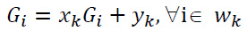
Medical imaging has developed a variety of denoising methods, including spatial domain, transform domain, and deep learning-based techniques, to suppress Gaussian noise interference in imaging, thereby enhancing imaging quality [18-20]. However, due to their simplicity and effective removal of specific types of noise, traditional spatial domain techniques for denoising, including Gaussian filtering, bilateral filtering, and median filtering, have been widely used in CT images. However, these methods often experience over-smoothing and the erosion of fine details. Conventional techniques frequently assume a uniform distribution of noise across the entire image. This assumption may not be effective in situations where noise levels vary in different regions. The higher noise regions can obscure structural and critical details, leading to degradation in imaging quality. Conversely, global denoising negatively impacts lower-noise regions, causing over-smoothing.overcome these issues, guided filtering has gained attention due to its ability to preserve edges while suppressing noise. The Guided filter is an edge-preserving filter primarily used for image denoising, smoothing, and enhancement [21]. It utilizes a guidance image to assist in smoothing while preserving crucial edges. The guided filter operates under the assumption that the relationship between guidance G and the guided filtering output  is linear. Suppose that is linear transformation of G in a window wk centered at pixel k, and it is expressed as shown in Eqs. (1, 2):
 |
(1) |
 |
(2) |
where,
i is the ith output image-pixel, Gi is the ith guidance image-pixel,
ni are the ith pixel noisy components,
qi is the input pixel at ith location, and (xk, yk) represents the certain linear coefficients considered to be constant in wk.
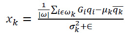
An input image q and the coefficients xk and yk are calculated within a local window ωk around each pixel i. The Coefficient xk is calculated as illustrated in Eq. (3):
 |
(3) |
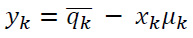
The Coefficient yk is calculated as expressed in Eq. (4) below:
 |
(4) |
where:
μk and
 are local means of q and G in the window (ωk),
σk2 - represents the variance of G in ωk,
|ω| - represents the number of pixels in ωk, and
∈ - is denoted as the regularization parameter to prevent division by zero.
The efficiency of the guided filter depends on the selection of the guidance image, the window size (radius), and the regularization factor (ϵ). It is highly useful for image smoothing and preserving sharp edges, making it a popular choice in various image processing tasks. Adaptive thresholding methods, in conjunction with various transform domain techniques such as wavelet, curvelet, tetrolet, and shearlet transforms, are effective for local noise estimation and denoising. These techniques decompose an image at multiple scales and orientations, providing a more detailed analysis of crucial image features and noise patterns. The wavelet transform is widely used for image denoising and enhances image quality due to its multi-resolution properties, sparsity, low entropy, decorrelation, and energy compaction. Wavelets are the mathematical functions that split the image into wavelet coefficients, capturing random variations at multiple scales and orientations. This allows for the separation of noisy coefficients from important details and the reduction of noise by applying thresholding to the noisy coefficients. Gabralla et al. proposed a methodology in which the Discrete Wavelet Transform (DWT) is applied to mitigate Gaussian noise in CT images [22]. However, the wavelet transform is prone to limited directionality and edge discontinuities, which can lead to inaccurate analysis of complex features like textures and edges.
Diwakar et al. introduced a methodology that identifies noise in CT images by analyzing a patch-based gradient approximation of the image and then reduces the noise using tetrolet transform with locally adaptive thresholding and nonlocal means filtering. This method effectively preserves crucial details and results in higher imaging quality. However, the tetrolets are not shift-invariant due to their discrete and block-based nature, which can cause inconsistencies and variations with small translations that occur in the image. Researchers have proposed multiscale and multi-directional geometric analysis methods, such as curvelet and shearlet transform, to overcome these limitations. Kamble et al. proposed a methodology in which the curvelet transform utilizes optimal sparsity, using fewer coefficients to represent images with edges, and anisotropic scaling, which scales differently along various axes to capture edges and curves effectively [23, 24]. The curvelet transform is specifically designed to capture image details along various directions and handles line singularities or curved features in order to represent edges and curves more efficiently. However, the limited directional representation of the curvelet transform fails to preserve crucial details.
Routray et al. suggested a methodology that the Shearlet-transform with bilateral filtering approach effectively suppresses noise while maintaining subtle features of an image [25]. The NSST is an advanced approach derived from the shearlet transform, extending the principles of the wavelet transform. It is constructed through an iterative application of atrous convolution methods combined with shearlet filters to ensure a shift-invariant multiscale and multidirectional decomposition process. NSST is derived from the classical theory of affine systems with multiple dilations and exhibits five key properties: good localization, spatial localization, high directional sensitivity, parabolic scaling, and optimal sparse representation. The NSST is achieved by combining the nonsubsampled laplacian pyramid transform with various shearing kernels. Unlike the traditional shearlet transform, NSST does not involve downsampling or upsampling, resulting in full shift-invariance, which helps to preserve finer image details during image processing tasks such as denoising. The shearlet transform can be represented in both continuous and discrete forms to preserve fine image details effectively. The continuous shearlet transform acts as a non-isotropic extension of the continuous wavelet transform with enhanced directional sensitivity. In the case of two dimensions (n=2), the continuous shearlet transform is expressed as a mapping function, allowing for the capture of directional information at multiple scales and orientations, making it effective for operations involving in-depth image analysis.
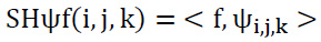
The dimensions of n=2, and for i>0, j∈R, k∈ R2. The shearlets can be expressed as illustrated in Eq. (5):
 |
(5) |
where,
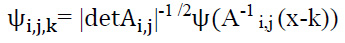
ψf(i,j,k) are referred to as shearlets. For i > 0, j∈R, k∈ R2, the shearlets could be evaluated as illustrated in Eq. (6):
 |
(6) |
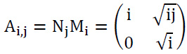
The matrix Ai,j can be factorized as shown in Eq. (7):
 |
(7) |
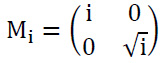
The anisotropic dilation can be described as illustrated in Eq. (8):
 |
(8) |
Where I>0, manages the scale of shearlets and provides frequency to acquire finer scales.
The shear matrix is obtained as shown in Eq. (9):
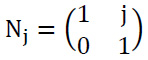 |
(9) |
Each matrix Ai,j is coupled with two different actions:
Anisotropic dilation resulting from the matrix Mi and shearing induced by the matrix Nj.
The direction of shearlets is controlled by the shear matrix. Therefore, the shearlet transform relies only on three variables, including scale i, orientation j, and location k. Ψ is a well localised function adhering to admissibility criteria.
For ξ0 = (ξ1,ξ2) ∈R2, ξ1≠ 0, let ψ be issued by using Eq. (10):
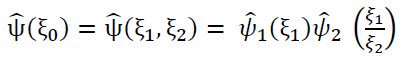 |
(10) |
where,
 is fourier transformation of
  is denoted as smooth functions characterized by their supports existing in [−2,−(1/2)] ∪ [1/2,2] and [−1,1], correspondingly. Subsequently, each f(x)∈S 2(R2) can be restored using the following formula (Eq. 11):
 |
(11) |
In the frequency domain, it is illustrated as (Eq. 12):
 |
(12) |
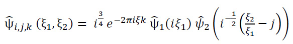
The support of each and every function
i,j,k is given by the following set (Eq. 13):
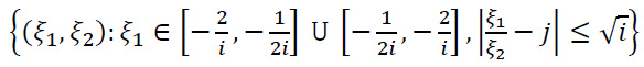 |
(13) |
Each shearlet ψi,j,k has frequency support on pairs of trapezoids at different scales, symmetrically around the origin, and aligned along a line with a slope determined by (j). As i→0, the support becomes thinner, allowing the shearlets to generate a group of precisely localized waveforms at multiple scales, orientations, and locations, managed by the parameters i, j, and k, correspondingly.
The discrete shearlet transform serves to illustrate multi-dimensional functions. These functions are generated by discretizing the scaling, shearing, and translation parameters. Specifically, i=2-2n,j=-L with n, k=P ∈Z2 and L ∈Z. This ensures the efficient representation of data across different scales, orientations, and positions in a discrete domain.
The discrete shearlet transformation can be expressed as given in Eq. (14):
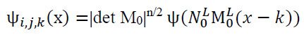 |
(14) |
where: M0 and N0 are associated with scaling and shear matrix can be denoted as given in Eq. (15):
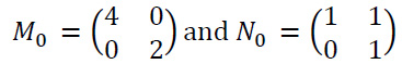 |
(15) |
From each function f ∈ L2 (R2), the provided method can be reconstructed by utilizing the properties of the function ψ as explained below in Eq. (16):
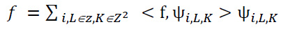 |
(16) |
Singh et al. proposed a methodology in which a new hybrid method employs a CNN with a method noise-based denoising approach to optimize the CT imaging quality [26]. This approach aims to recover lost information during the noise reduction process. The aim of the technique is to utilize the method of noise to recognize noisy patterns and refine the denoising process. The CNN effectively learns to eliminate noise patterns while conserving significant features and edges in the images. However, the performance of the method noise-based DnCNN approach is sensitive to hyperparameter tuning such as thresholding value and learning rate. Diwakar et al. proposed a methodology in which a noise reduction technique using the Bayes shrinkage rule in the shearlet domain performs noise suppression and fine detail preservation effectively [27]. The multiscale and multidirectional features of the shearlet transform allow for the identification of noisy coefficients by estimating the optimal threshold value based on noise features and statistical properties, thereby ensuring effective noise suppression in CT images.
Kumar et al. suggested a hybrid approach that combines the NSST with SURELET and a wiener filter for effective denoising of CT images [28]. The shearlet transform captures multiscale and multi-directional features from the noisy image. The thresholding function SURELET is used to adaptively threshold the image’s noise coefficients, depending on an unbiased estimate relating to the Mean Squared Error (MSE). The main aim of SURELET is to minimize MSE by choosing the optimal threshold value for noise mitigation while maintaining the fine details of images. The Wiener filter is applied to the shearlet coefficients to suppress noise by using local variance, which adaptively sets the strength of the Wiener filter to achieve optimal noise suppression. Finally, combining the NSST transform with Wiener filtering helps to maintain image details and diminish artifacts. Kumar et al. [29] suggested a method in which the tetrolet transform is applied on noisy CT images, employing a locally adaptive shrinkage method on high-frequency components to effectively suppress noise, particularly in smooth regions with geometric features. However, the tetrolet transform fails to capture edge details, as well as multidirectional and anisotropic features of LDCT images, which are crucial for effective noise suppression.
Abuya et al. proposed a methodology in which an Anisotropic Gaussian Filter (AGF) and the Haar wavelet transform are suggested as preprocessing steps, while a deep learning-based Denoising CNN (DnCNN) framework is used as a postprocessing step to mitigate any residual noise in CT images [30]. The ability of AGF to depict edge orientation and directional information helps to reduce edge blurriness in CT images, especially when the noise is distributed in a non-uniform manner. The method ensures better noise suppression, although it might cause a loss of fine image details in highly textured (edge) regions, which can degrade diagnostic accuracy.
In recent decades, deep learning techniques have proven remarkable results in addressing CT denoising issues. Yang et al. suggested a methodology that includes a deep CNN for image denoising, which preserves critical diagnostic information by assessing the perceptual features of the ground truth and denoised images in image feature space rather than using mean squared error [31]. Unlike traditional methods, which focus on minimizing mean squared error through pixel-to-pixel variations, often resulting in the over-smoothing of images, the new method focuses on perceptual features, thereby preserving important structural details for precise medical diagnosis. However, the implementation of deep learning models and feature space comparisons can lead to computational overhead. Wu et al. proposed a methodology to enhance the diagnostic accuracy of LDCT images using adaptive edge prior and deep learning Cross Scale Residual Channel Attention Network framework (RCA-Net) to suppress Gaussian noise while maintaining edge details and lesion characteristics in CT images [32]. The adaptive edge prior is combined into the network to preserve the integrity of image boundaries and unique image features. Additionally, Cross Scale Mapping And A Dual-Element Module (CMDM) are used to maintain complex edge patterns during training, helping the model to distinguish between edge textures and lesion regions. The novel compound loss function integrates mean squared error with multiscale-attention-residual perception-loss to mitigate excessive smoothing of denoised CT images. However, complexity may arise in the implementation of adaptive edge priors and the CMDM framework, and the use of multiple models can result in longer training times.
Zhang et al. proposed a deep CNN framework, which is accompanied by the shearlet transform and a Denoising Autoencoder (DAE) to minimize noise in CT images and enhance image quality [33]. Initially, the author uses the shearlet transform to split the image into low and high-frequency coefficients, then analyzes the image at various scales and orientations to identify and suppress different noise levels. After the shearlet transform, DAE is applied to the transformed coefficients to further mitigate noise. The DAE consists of an encoder-decoder network. The encoder compresses the original image into a lower-dimensional (more concise) latent representation, while the decoder reconstructs the image from this representation. The autoencoder is trained using pairs of low- high-quality images to learn how to transform noisy images into clean images, helping the model effectively extract structural information and suppress noise. The decoding process reconstructs the final denoised image from the processed coefficients, effectively mitigating noise to achieve a superior image. The combination with respect to the shearlet transform and DAE not only preserves edges but also effectively suppresses noise in LDCT images. However, this method relies heavily on the quality of preprocessing operations, such as noise suppression and initial image orientation, which can affect overall denoising performance. Recently, transformer models have also played a significant role in noise suppression for CT images.
Zhang et al. proposed a hybrid denoising technique that incorporates transformer models with CNNs to enhance the quality of tomographic images [34]. The transformer identifies long-distance dependencies and global contextual information throughout the whole image, while the CNN extracts local spatial attributes and fine details. The combination of the CNN’s ability to extract local features (including noise) and the transformer’s capability to retain global dependencies leads to improved denoising performance.
Zhang et al. proposed a methodology that incorporates the Denoising Swin Transformer model (DnST), which integrates a modified Shifted Window (SWIN) Transformer with perceptual loss and a residual-mapping process to enhance denoising [35]. Perceptual PSNR (PPSNR) is leveraged to measure the perceptual traits of the image, comparing them with the ground (baseline)truth in feature space to assess CT imaging quality. The SWIN transformer architecture is ideal for handling complex structures and textures in various types of LDCT imaging, outperforming traditional CNN models. However, the model’s success highly relies on large, labeled datasets of noisy and clean CT images for training.
Zubair et al. proposed a methodology that incorporates the Difference of Gaussian (DoG) Sharpening layer in the network, which enhances features at different scales based on the DoGs and utilizes attention mechanisms to focus on important details, thereby improving the clinical detection rate [36]. This approach efficiently suppresses noise while conserving image details. However, the model’s interpretational complexity, associated with higher resource consumption, may hinder its applicability in real-time healthcare environments. Zubair M et al. proposed EdgeNet+, a variant of U-Net with 21 convolutional layers and three skip connections, designed to capture structural information for noise suppression and image refinement [37]. It employs a multi-stage edge detection block at a deeper level and utilizes a loss function combining SSIM and L1 losses to improve detection accuracy. EdgeNet+ demonstrates enhanced noise suppression and artifact removal, producing denoised CT images that closely resemble normal-dose CT images. However, the integration of advanced techniques might complicate implementation and require specialized expertise.
A recent approach, the hybrid Attention-Guided enhanced U-Net with hybrid edge-preserving structural loss, has been developed for LDCT image denoising [38]. It utilizes residual blocks for key detail detection, attention gates to enhance the upsampling process, and a custom hybrid loss that combines structural loss with Euclidean norm gradient regularization. This method achieves a PSNR of 39.65, an SSIM of 0.91, and an RMSE of 0.016 but requires high computational resources. In contrast, the proposed method integrates NSST, an edge-guided filter, and a method noise approach. NSST ensures multi-directional analysis, the edge-guided filter preserves edge details, and method noise enhances structural details, yielding superior image quality while preserving diagno -stic accuracy.
3. PROPOSED METHODOLOGY
The overall process is introduced as follows:
This method combines NSST, guided filtering, the BayesShrink method, and residual processing for effective noise mitigation in medical imaging, which is often corrupted by Gaussian noise [39]. The proposed approach is segmented into two primary stages. In the first stage, initial denoising is performed using the NSST approach, guided filtering, and the BayesShrink thresholding method. In the second stage, residual processing is applied to further suppress noise and preserve fine image details.
3.1. The Proposed Algorithm
Input: Noisy CT image X'n.
Output: Denoised CT image X'f.
3.1.1. Gaussian Noise
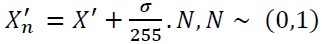
Initially, Gaussian noise is introduced to the clean image (X'), and it is expressed as (Eq. 17):
 |
(17) |
X'n is the resulting noisy image,
 is the noise scaling factor, σ represents the noise standard deviation, and
N is the noise component, usually Gaussian noise, which is incorporated to clean the image.
3.1.2. Noisy Input
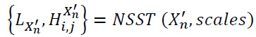
For a noisy input image Xn′X_n'Xn′, decompose the image using the NSST approach with a low-pass filter and specific shear parameters to obtain (Eq. 18):
 |
(18) |
where,
i represents the scale level,
j represents the directional component, and
scales represent the number of decomposition levels.
3.1.3. Apply Filtering
Apply guided filtering to the low-frequency components(approximation) LX'n based on the parameters r = 4 (filter radius) ϵ = 0.012 (degree of smoothing) to obtain the filtered image LfX'n as described in Eqs. (3 and 4) and shown in Eq. (19):
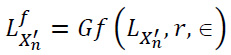 |
(19) |
Process the neighborhood pixels by applying the max rule on decomposed low-frequency components LX'n of the input images, depending on the average of 3x3 neighborhood pixels.
3.1.4. Decomposition Level
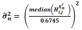
For each decomposition level, i do For each orientation j do Process the high-frequency components Hi,jX'n by applying the BayesShrink method to assess the noise and signal variance.
The noise variance can be expressed as (Eq. 20):
 |
(20) |
The signal variance can be expressed as given in Eq. (21) below:
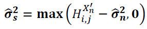 |
(21) |
Calculate the BayesShrink threshold value using the following formula (Eq. 22):
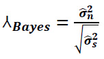 |
(22) |
Apply thresholding to the high-frequency noisy components Hi,jX'n to obtain the filtered approximation details, as expressed in Eq. (23):
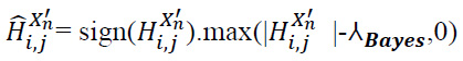 |
(23) |
end for (j)
end for (i)
3.1.5. Combine Components
Combine the filtered low-frequency components and thresholded high-frequency components to reconstruct the denoised CT image X'rec as illustrated in Eq. (24):
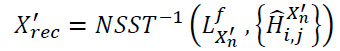 |
(24) |
3.1.7. Apply Decomposition
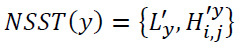
Apply NSST decomposition to the residual image y.
The decomposition process of residuals is shown in Eq. (26):
 |
(26) |
where,
L'y illustrates the low-frequency components of residual image y after the NSST process and
 represents the high-frequency components of residual image y after the NSST process.
3.1.8. Repeat Thresholding
Repeat the BayesShrink thresholding method on high-frequency (detail) components of residual
using step 4.
3.2. Proposed Approach
The core steps of the proposed algorithm are outlined in Fig. (1), which demonstrates the structure of the proposed method. A detailed explanation of the proposed methodology is provided in the following section.
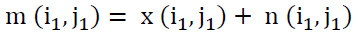
Assuming that CT images are frequently compromised by Additive White Gaussian Noise (AWGN) featuring zero mean and standard deviation (σ), variance σ2n, the noisy image can be mathematically represented as expressed in Eq. (29):
 |
(29) |
where:
m (i1, j1) represents the noisy image,
x (i1, j1) - illustrates the clean image, and
n (i1, j1) – illustrates the Gaussian noisy coefficients.
3.3. Proposed Algorithm Explanation
The proposed approach consists of two stages. In the first stage, the generalized NSST approach is applied to the CT image X', which contains Gaussian noise, resulting in a noisy version X'n. The image X'n is decomposed by NSST to low and high-frequency components {LX'n,Hi,jX'n} at decomposition level i and direction j. The number of decomposition levels n plays a crucial role in the denoising process. Typically, low-frequency components capture the overall intensities of the input images, while high-frequency components represent variations across different scales and directions. The low-frequency components, which contain smoother regions, are processed using guided filtering. Meanwhile, the high-frequency components, which include edges and fine details, are processed using the BayesShrink thresholding method to suppress noise without degrading image quality. This results in the denoised low-frequency components LfX'n and the denoised high-frequency components
 . The final denoised image X'rec is obtained by applying the inverse NSST to reconstruct the image.
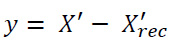
In the second stage, residual image y is used to capture discrepancies between the noisy image and the denoised image. This residual image isolates the noise that was removed during the denoising process, further enhancing the overall image quality. The NSST is reapplied to the residual image to decompose it into coarse (low-frequency) components (L'y) and fine (high-frequency) components (
). The low-frequency components represent smooth structures, such as basic shapes and gradients, while the high-frequency components capture sharp features like edges and textures. The high-frequency components of the residual image are further processed using BayesShrink thresholding to obtain denoised coefficients. The residuals are then reconstructed using the inverse NSST process.
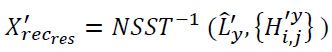
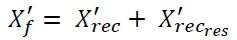
Finally, the overall final denoised image (X'f) is obtained by combining the initially reconstructed denoised image (X'rec) with the reconstructed residual image (X'recrec). This combination enhances noise suppression while preserving important diagnostic details in the CT images. This novel two-stage denoising process effectively alleviates both low and high-frequency noise components, ultimately improving image quality for more accurate medical interpretation.
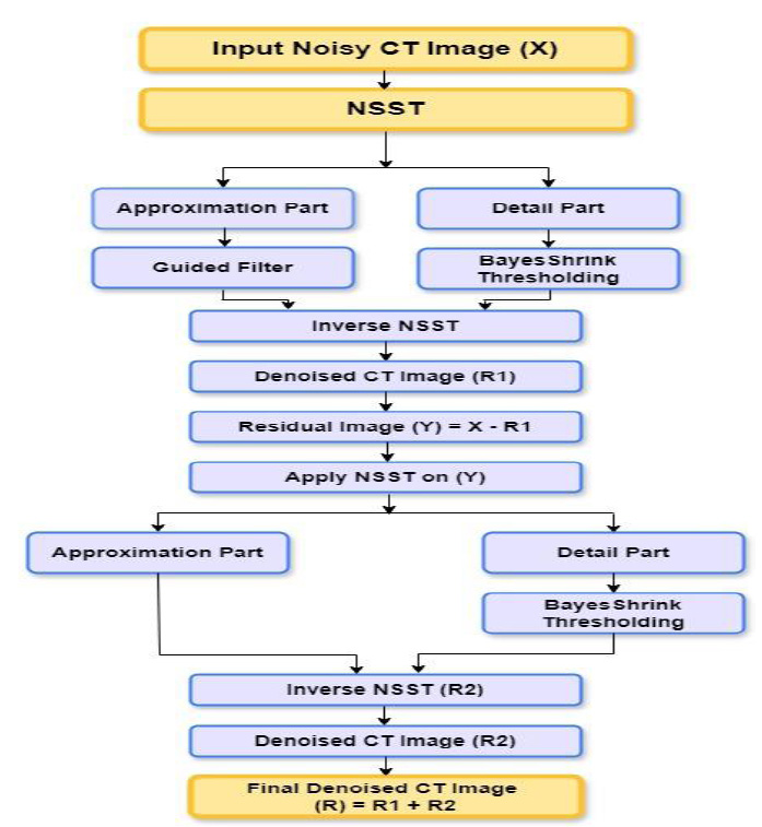
Flowchart of the proposed denoising method.
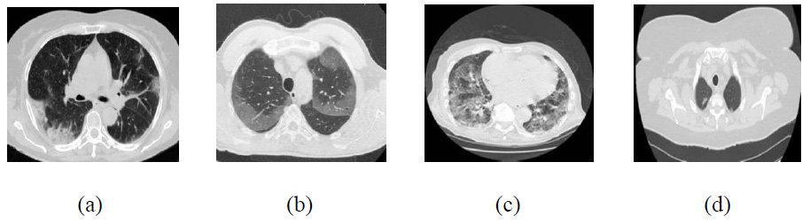
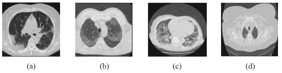
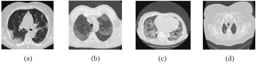
Clean CT images.
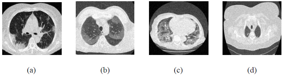
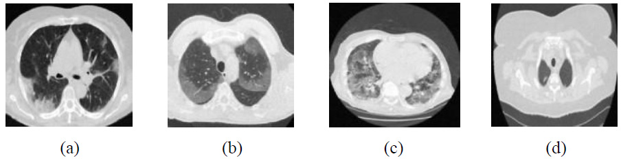
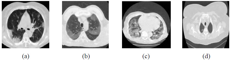
Noisy CT images at noise variance σ =10.
4. THE EXPERIMENTAL RESULTS AND DISCUSSION
The existing denoising methods, along with the newly proposed method, are applied to various Gaussian noisy CT images to validate the method’s efficiency. The grayscale CT images, with a resolution of 512x512 pixels, are acquired from the “Large COVID-19 CT scan slice dataset.” The experiments on Gaussian noisy images allow for validating the proposed method in terms of noise suppression and edge preservation capabilities. The clean CT images (CT1, CT2, CT3, and CT4) are shown in Fig. (2), while Additive Gaussian noisy images with a noise-variance of σ = 10 are depicted in Fig. (3).
A systematic technique was implemented for an in-depth analysis of the effectiveness of various denoising methods while compensating for possible variations. Gaussian noise was introduced into the CT images at different noise variance levels, ranging from 5 to 20. The primary focus of these denoising implementations was to mitigate Gaussian blur noise and preserve edges across diverse noise levels, thereby evaluating the denoising effectiveness and assessing CT image quality.
4.1. Quantitative Analysis metrics
The proposed method was verified through various existing denoising methods. The quantitative performance evaluation metrics like Peak Signal-to-Noise Ratio (PSNR), Structural Similarity Index Measure (SSIM), Entropy Difference (ED), Feature Similarity Index Measure (FSIM), and Root Mean Squared Error (RMSE) were implemented to measure the experimental result. The proposed method NSST with BayesShrink thresholding and guided filtering were evaluated in conjunction with other modern denoising methods using PSNR, SSIM, ED, FSIM, and RMSE as standard measures of quantity as shown below [40, 41].
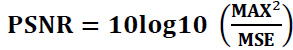
4.1.1. Peak-Signal-to-Noise-Ratio (PSNR):
It is used to evaluate the quality of denoised images compared to original images. PSNR measures the ratio of the maximum power of a signal and the power of noise or distortion affecting the signal.
For the input CT image P and the denoised CT image Q,
PSNR is expressed as folllows (Eq. 30):
 |
(30) |
Here, MSE can be calculated as follows (Eq. 31):
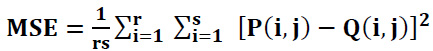 |
(31) |
where,
MAX illustrates the maximum grayscale value in the image,
MSE stands for the mean-squared error between the original image and the denoised CT image,
P (i, j) represents the clean CT image,
Q(i, j) represents the denoised or filtered CT image, and r x s indicates the size of the pixel of the original image and processed or denoised CT image.
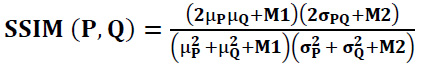
4.1.2. Structural-Similarity-Index-Measure (SSIM):
It is used to assess the similarity between two images i.e. the perceptual quality of an image based on structural details and visual interpretation aspects including contrast, brightness, and structural details.
The range of SSIM value between -1 and 1, in which 1 denotes perfect similarity, -1 implies dissimilarity between two images, and 0 indicates no structural correlation between images (Eq. 32):
 |
(32) |
where,
P denotes clean CT image and
Q denotes denoised CT image.
µP
µQ
are represented as the local-means
 are denoted as variances of P and Q, and σPQ covariance of the image’s P and Q. Here, M1=(x1C)2 and M2=(x2C)2 are stabilizing factors for division with zeros, where C is the dynamic range of pixel brightness values between 2bits-per-pixel-1 and 1. Here, x1 and x2 are constant values x1= 0.01 & x2 = 0.03.
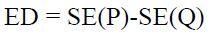
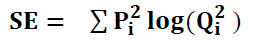
4.1.3. Entropy Difference (ED)
The Entropy Difference is the statistical noise metric to measure the amount of randomness or information in the image, that helps in analyzing the texture patterns of the given input images. Shannon entropy is calculated in comparison to the original image (P) and the denoised CT image (Q). The mean value discrepancy is illustrated as ED. ED is computed as demonstrated in Eq. (33):
 |
(33) |
where:
SE denotes the Shannon entropy.
Shannon Entropy is calculated as given in Eq. (34):
 |
(34) |
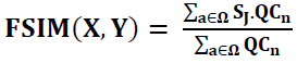
4.1.4. Feature Similarity Index Measure (FSIM):
Feature-similarity-index-measure is a visual quality performance benchmark for evaluating the congruence of the denoised image with the clean image with regard to its structural features. The FSIM is derived from the way the human visual system primarily interprets an image, which is influenced by its low-level features.
The FSIM is calculated using the following formula (Eq. 35):
 |
(35) |
where:
Ω represents the total image space or domain, and also, Sj = SQC.SH and QCn = max(QC1.QC2). Here, SQC, which represents the phase congruency similarity, can be expressed as (Eq. 36):
 |
(36) |
SH, which represents gradient magnitude similarity can be expressed as (Eq. 37):
 |
(37) |
where:
QC1 and QC2 denote phase congruency-maps and H1 and H2 denote gradient magnitude maps. T1 is used to represent small positive constants to improve the stability of SQC. The T1 is assessed based on the dynamic range of QC values, while T2 represents a positive constant based on the dynamic range of gradient magnitude values. For the experiments, the values were set to T1=0.85 and T2=160.
4.2. The quantitative result analysis
The performance of the proposed method was validated and tested by comparing the different Gaussian noisy CT-based images with other existing denoising methods. The CT images CT1, CT2, CT3, and CT4 were used to compare the proposed method with different denoising techniques for noise variance (σ=5,10,15,20). The comparisons of proposed ensembled method with other denoising approaches, such as Discrete Wavelet Transform [22], NSST with bilateral filter [25], method noise-based CNN [26], NSST with Bayes Shrinkage [27], NSST with wiener filtering and SURELET [28], Tetrolet transform [29], and their performance in terms of PSNR, SSIM, ED, FSIM and RMSE are displayed in Tables 1-4. The graphical comparison of PSNR, SSIM, ED, FSIM, and RMSE values of different denoising schemes and the proposed approach for CT image are depicted in Figs. (4-8).
The best experimental outcomes are shown in bold. The experimental outcomes displayed in the tables validate the excellence of the proposed method among other existing denoising methods. The experimental outcome of the PSNR values of the proposed method, compared to other denoising methods, are shown in Table 1. The proposed hybrid method shows the best results among the compared methods. Generally, if the PSNR value is low, the restored imaging quality could be better. It was observed that the NSST with the Bilateral filtering method [25] at σ = 10 in the CT4 image depicts the best performance relative to all other methods, even though the complete texture of the proposed method is better at σ = 10 in the CT4 image. Overall, in CT images 1- 4, the proposed method shows the best outcomes at various noise levels, improving imaging quality.
The comparisons of the proposed ensembled method with other denoising approaches and their performance in terms of SSIM values are illustrated in Table 2. The proposed method’s SSIM values yield the superior results among all the compared methods. The resulting SSIM value falls within the range of 0 and 1. Here,1 denotes perfect similarity, 0 illustrates no similarity, and -1 illustrates perfect anti-correlation. It was noted that the proposed approach offers the best results with the resultant SSIM values between 0 to 1.
| Image | σ | PSNR | ||||||
|---|---|---|---|---|---|---|---|---|
| Discrete Wavelet Transform [22] | NSST with Bilateral [25] | Method noise-based CNN [26] | NSST with Bayes shrinkage [27] | NSST with Wiener Filter and SURELET [28] | Tetrolet Transform [29] | Proposed | ||
| CT 1 | 5 | 36.24 | 33.85 | 28.19 | 31.42 | 27.63 | 36.14 | 40.52 |
| 10 | 31.90 | 33.54 | 22.43 | 29.68 | 21.67 | 31.93 | 37.77 | |
| 15 | 29.40 | 33.00 | 19.15 | 28.53 | 18.38 | 2.231 | 36.41 | |
| 20 | 27.49 | 32.20 | 17.79 | 27.72 | 17.13 | 27.25 | 34.17 | |
| CT 2 | 5 | 36.59 | 35.16 | 26.76 | 32.11 | 28.36 | 37.05 | 39.17 |
| 10 | 32.62 | 34.80 | 22.76 | 30.70 | 26.96 | 32.49 | 35.20 | |
| 15 | 29.91 | 34.16 | 18.93 | 29.71 | 18.56 | 29.64 | 34.99 | |
| 20 | 27.93 | 33.24 | 16.31 | 28.92 | 15.99 | 27.51 | 33.95 | |
| CT 3 | 5 | 37.00 | 34.27 | 28.25 | 33.51 | 28.05 | 37.00 | 40.53 |
| 10 | 32.57 | 33.97 | 21.87 | 31.27 | 22.51 | 32.57 | 35.67 | |
| 15 | 29.97 | 33.41 | 19.89 | 29.85 | 19.48 | 29.97 | 36.12 | |
| 20 | 28.18 | 32.59 | 17.70 | 28.70 | 16.22 | 28.18 | 34.46 | |
| CT 4 | 5 | 37.74 | 37.32 | 27.84 | 35.51 | 26.85 | 37.74 | 41.05 |
| 10 | 33.11 | 36.70 | 22.02 | 33.66 | 21.55 | 33.11 | 36.02 | |
| 15 | 30.17 | 35.72 | 18.07 | 32.44 | 17.80 | 30.17 | 38.00 | |
| 20 | 28.17 | 34.36 | 16.35 | 31.10 | 15.96 | 28.17 | 36.30 | |
| Image | σ | SSIM | ||||||
|---|---|---|---|---|---|---|---|---|
| Discrete Wavelet Transform [22] | NSST with Bilateral [25] | Method noise-based CNN [26] | NSST with Bayes shrinkage [27] | NSST with Wiener Filter and SURELET [28] | Tetrolet Transform [29] | Proposed | ||
| CT 1 | 5 | 0.6491 | 0.9113 | 0.9054 | 0.8460 | 0.9019 | 0.9157 | 0.9698 |
| 10 | 0.4970 | 0.9011 | 0.8673 | 0.8128 | 0.7693 | 0.7949 | 0.9381 | |
| 15 | 0.4070 | 0.8839 | 0.8196 | 0.7874 | 0.6195 | 0.6746 | 0.9138 | |
| 20 | 0.3443 | 0.8552 | 0.7807 | 0.7588 | 0.4903 | 0.5708 | 0.9201 | |
| CT 2 | 5 | 0.6380 | 0.9208 | 0.8961 | 0.8581 | 0.9030 | 0.9173 | 0.9503 |
| 10 | 0.4735 | 0.9148 | 0.8682 | 0.8379 | 0.7514 | 0.7950 | 0.9287 | |
| 15 | 0.3651 | 0.9007 | 0.8204 | 0.8215 | 0.5841 | 0.6646 | 0.9089 | |
| 20 | 0.2942 | 0.8736 | 0.7766 | 0.7928 | 0.4567 | 0.5503 | 0.8953 | |
| CT 3 | 5 | 0.5487 | 0.9305 | 0.8875 | 0.8814 | 0.9141 | 0.9110 | 0.9486 |
| 10 | 0.4204 | 0.9084 | 0.8511 | 0.8455 | 0.7556 | 0.7680 | 0.9123 | |
| 15 | 0.3458 | 0.8763 | 0.8031 | 0.8153 | 0.5940 | 0.6324 | 0.9124 | |
| 20 | 0.2956 | 0.8334 | 0.7965 | 0.7740 | 0.4676 | 0.5245 | 0.8854 | |
| CT 4 | 5 | 0.4657 | 0.9596 | 0.8951 | 0.9252 | 0.9089 | 0.9173 | 0.9677 |
| 10 | 0.3231 | 0.9466 | 0.8631 | 0.9063 | 0.7274 | 0.7701 | 0.9498 | |
| 15 | 0.2459 | 0.9228 | 0.8158 | 0.8863 | 0.5560 | 0.6247 | 0.9414 | |
| 20 | 0.2020 | 0.8852 | 0.7811 | 0.8373 | 0.4304 | 0.5040 | 0.9243 | |
| Image | σ | ED | ||||||
|---|---|---|---|---|---|---|---|---|
| Discrete Wavelet Transform [22] | NSST with Bilateral [25] | Method noise-based CNN [26] | NSST with Bayes shrinkage [27] | NSST with Wiener Filter and SURELET [28] | Tetrolet Transform [29] | Proposed | ||
| CT 1 | 5 | 0.1257 | 0.1699 | 0.1762 | 0.1221 | 0.1440 | 0.1972 | 0.1183 |
| 10 | 0.1676 | 0.2497 | 0.2181 | 0.2260 | 0.1753 | 0.1775 | 0.1745 | |
| 15 | 0.2007 | 0.2977 | 0.2954 | 0.3024 | 0.1817 | 0.1472 | 0.1413 | |
| 20 | 0.2093 | 0.3214 | 0.3698 | 0.3362 | 0.1909 | 0.1509 | 0.1503 | |
| CT 2 | 5 | 0.1636 | 0.2224 | 0.2677 | 0.2625 | 0.2271 | 0.1882 | 0.1564 |
| 10 | 0.2758 | 0.3701 | 0.3039 | 0.4332 | 0.2786 | 0.2698 | 0.2692 | |
| 15 | 0.2993 | 0.4630 | 0.4947 | 0.5516 | 0.3196 | 0.2458 | 0.2400 | |
| 20 | 0.2995 | 0.4871 | 0.6424 | 0.5971 | 0.3283 | 0.2531 | 0.2942 | |
| CT 3 | 5 | 0.1970 | 0.3119 | 0.1953 | 0.4091 | 0.2093 | 0.1956 | 0.1910 |
| 10 | 0.2839 | 0.4219 | 0.3224 | 0.6017 | 0.2248 | 0.2273 | 0.2244 | |
| 15 | 0.3144 | 0.4635 | 0.4365 | 0.6996 | 0.2422 | 0.2466 | 0.2399 | |
| 20 | 0.2776 | 0.4225 | 0.5020 | 0.6647 | 0.1679 | 0.2523 | 0.2695 | |
| CT 4 | 5 | 0.2612 | 0.5259 | 0.2693 | 0.4210 | 0.3100 | 0.2712 | 0.2602 |
| 10 | 0.3811 | 0.7040 | 0.4685 | 0.6438 | 0.2837 | 0.3066 | 0.3027 | |
| 15 | 0.4420 | 0.8004 | 0.6184 | 0.7952 | 0.3118 | 0.3564 | 0.3102 | |
| 20 | 0.4784 | 0.7964 | 0.7494 | 0.8137 | 0.3273 | 0.3624 | 0.3258 | |
| Image | σ | FSIM | ||||||
|---|---|---|---|---|---|---|---|---|
| Discrete Wavelet Transform [22] | NSST with Bilateral [25] | Method noise-based CNN [26] | NSST with Bayes shrinkage [27] | NSST with Wiener Filter and SURELET [28] | Tetrolet Transform [29] | Proposed | ||
| CT 1 | 5 | 0.9882 | 0.9979 | 0.9980 | 0.9850 | 0.9930 | 0.9998 | 0.9999 |
| 10 | 0.9658 | 0.9978 | 0.9994 | 0.9781 | 0.9858 | 0.9991 | 0.9995 | |
| 15 | 0.9409 | 0.9977 | 0.9989 | 0.9729 | 0.9812 | 0.9979 | 0.9990 | |
| 20 | 0.9139 | 0.9975 | 0.9983 | 0.9702 | 0.9784 | 0.9960 | 0.9985 | |
| CT 2 | 5 | 0.9847 | 0.9971 | 0.9996 | 0.9812 | 0.9892 | 0.9995 | 0.9997 |
| 10 | 0.9961 | 0.9973 | 0.9985 | 0.9762 | 0.9830 | 0.9978 | 0.9989 | |
| 15 | 0.9327 | 0.9969 | 0.9979 | 0.9731 | 0.9800 | 0.9949 | 0.9981 | |
| 20 | 0.9038 | 0.9964 | 0.9966 | 0.9702 | 0.9774 | 0.9908 | 0.9970 | |
| CT 3 | 5 | 0.9862 | 0.9968 | 0.9985 | 0.9791 | 0.9891 | 0.9989 | 0.9993 |
| 10 | 0.9587 | 0.9969 | 0.9986 | 0.9686 | 0.9817 | 0.9972 | 0.9987 | |
| 15 | 0.9282 | 0.9966 | 0.9965 | 0.9615 | 0.9803 | 0.9937 | 0.9975 | |
| 20 | 0.8997 | 0.9959 | 0.9963 | 0.9585 | 0.9778 | 0.9892 | 0.9969 | |
| CT 4 | 5 | 0.9837 | 0.9976 | 0.9991 | 0.9719 | 0.9825 | 0.9987 | 0.9990 |
| 10 | 0.9490 | 0.9967 | 0.9960 | 0.9659 | 0.9786 | 0.9941 | 0.9971 | |
| 15 | 0.9088 | 0.9960 | 0.9954 | 0.9644 | 0.9802 | 0.9880 | 0.9966 | |
| 20 | 0.8711 | 0.9935 | 0.9936 | 0.9629 | 0.9805 | 0.9811 | 0.9948 | |
For example, in CT images, values such as 1, 2, 3, and 4 that are very close to 1 indicate an almost perfect similarity between the original image and the denoised image.
The ED values of the various existing denoising methods and the proposed method are depicted in Table 3. However, the proposed method gives better-denoised results indicating low entropy difference in CT images. The entropy difference measures the amount of randomness in the CT images. Higher ED values indicate a lot of noise or detail, while lower ED values suggest smooth areas in CT images. Table 3 reveals that the Discrete Wavelet Transform method achieves higher entropy values at σ=10 in the CT1 image, while the Tetrolet Transform shows lower ED values. At σ=20, the NSST method combined with Wiener filtering and the SURELET approach achieved optimal results in CT3 and CT4 [22, 28, 29]. Although these methods show slightly lower entropy difference values in some cases, the proposed method consistently demonstrates better denoising performance. The FSIM values of the proposed method, along with other existing denoising methods, are depicted in Table 4. It is demonstrated that the proposed approach excels over other denoising approaches in terms of FSIM values by comparing with other existed methods. The FSIM aligns more closely with human visual perception, providing a clearer assessment of denoising effectiveness.
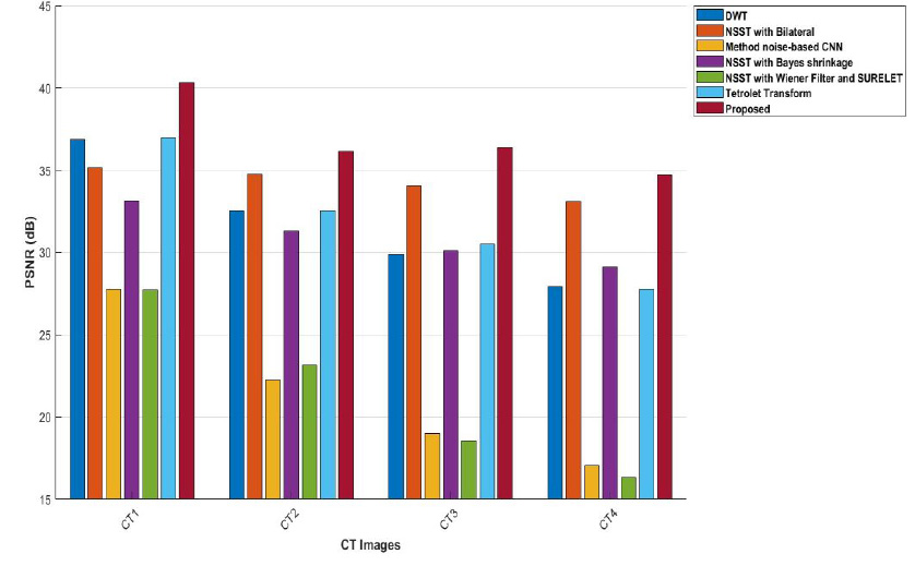
Graph comparison of PSNR values of various denoising schemes and the proposed method for CT images CT1, CT2, CT3, and CT4.
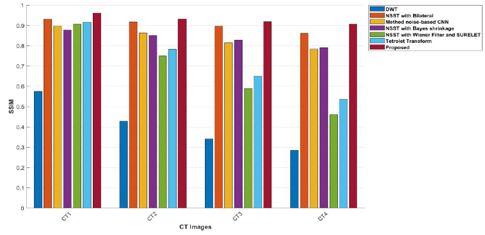
Graphical notation of SSIM values at various noise variance intensities from 5 to 20.
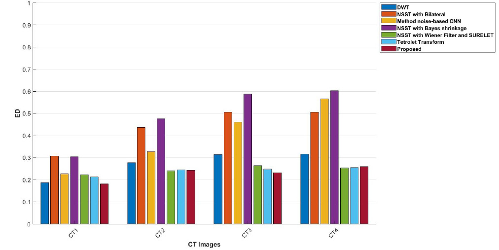
Graphical representation of a comparison of ED values of CT images CT1, CT2, CT3, and CT4 using the proposed method and other denoising schemes.
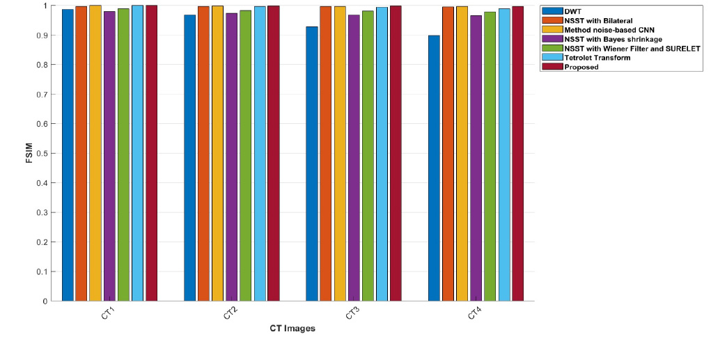
Graph comparison of FSIM values of various denoising schemes and the proposed method for CT images CT1, CT2, CT3, and CT4.
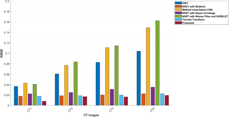
Graph comparison of RMSE values of various denoising schemes and the proposed method for CT images-CT1, CT2, CT3, and CT4.
The RMSE values of the proposed method, in comparison with other denoising approaches, are shown in Table 5. The proposed method depicts the best performance in suppressing noise and achieving the lowest RMSE values across various noise levels. RMSE is used to measure pixel-wise differences between the input clean images and the denoised images. A lower RMSE value denotes superior denoising performance. For example, with the noise intensity level of σ = 5, RMSE values 0.0092 for the CT3 image and 0.0008 for the CT4 image, outperforming all other noise levels. Among NSST-based techniques, NSST with a Bilateral filter can be considered competitive but less efficient, having an RMSE of 0.0136 in the CT4 image at σ = 5 [25]. Analyzing the results, the Discrete Wavelet Transform (DWT) is less effective compared to the Tetrolet transform, especially at high noise levels, with an RMSE of 0.0219 of CT2 at σ=20. Overall, the proposed method is superior to existing denoising methods in improving image quality [22, 29].
| Image | σ | RMSE | ||||||
|---|---|---|---|---|---|---|---|---|
| Discrete Wavelet Transform [22] | NSST with Bilateral [25] | Method noise-based CNN [26] | NSST with Bayes shrinkage [27] | NSST with Wiener Filter and SURELET [28] | Tetrolet Transform [29] | Proposed | ||
| CT 1 | 5 | 0.0399 | 0.0203 | 0.0419 | 0.0261 | 0.0408 | 0.0203 | 0.0118 |
| 10 | 0.0655 | 0.0211 | 0.0866 | 0.0329 | 0.0869 | 0.0210 | 0.0182 | |
| 15 | 0.0875 | 0.0223 | 0.1114 | 0.0374 | 0.1080 | 0.0224 | 0.0189 | |
| 20 | 0.1100 | 0.0246 | 0.1559 | 0.0412 | 0.1887 | 0.0245 | 0.0222 | |
| CT 2 | 5 | 0.0377 | 0.0175 | 0.0375 | 0.0248 | 0.0358 | 0.0175 | 0.0109 |
| 10 | 0.0599 | 0.0182 | 0.0748 | 0.0292 | 0.0947 | 0.0182 | 0.0172 | |
| 15 | 0.0819 | 0.0196 | 0.1087 | 0.0323 | 0.1146 | 0.0195 | 0.0177 | |
| 20 | 0.1018 | 0.0217 | 0.1678 | 0.0356 | 0.1594 | 0.0219 | 0.0201 | |
| CT 3 | 5 | 0.0366 | 0.0194 | 0.0399 | 0.0210 | 0.0425 | 0.0194 | 0.0092 |
| 10 | 0.0609 | 0.0200 | 0.0672 | 0.0272 | 0.0677 | 0.0201 | 0.0164 | |
| 15 | 0.0833 | 0.0214 | 0.1067 | 0.0321 | 0.1229 | 0.0213 | 0.0158 | |
| 20 | 0.1034 | 0.0235 | 0.1234 | 0.0370 | 0.1304 | 0.0236 | 0.0190 | |
| CT 4 | 5 | 0.0332 | 0.0136 | 0.0540 | 0.0168 | 0.0450 | 0.0136 | 0.0008 |
| 10 | 0.0570 | 0.0146 | 0.0817 | 0.0121 | 0.0863 | 0.0147 | 0.0157 | |
| 15 | 0.0782 | 0.0165 | 0.1173 | 0.0240 | 0.1133 | 0.0164 | 0.0126 | |
| 20 | 0.1020 | 0.0194 | 0.1494 | 0.0278 | 0.1716 | 0.0192 | 0.0153 | |
The experimental results are tested over different noise levels, but visual results are depicted only at noise intensity level 10. The analysis of the experimental output images in Figs. (9-15), unveiled that the proposed approach excels beyond other methods in the context of noise suppression and edge retention of significant image details.
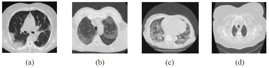
The experimental outcomes of CT images using the discrete wavelet transform are shown in Fig. (9) [22]. This method shows that at low noise intensity (σ=5), it results in moderate PSNR values ranging from 36 to 38 dB. Overall, CT images depict moderate denoising effectiveness at mild noise intensity levels. However, the proposed approach consistently achieves 3-4 dB at higher PSNR values across all noise intensities than DWT [22]. As the noise intensity levels increase (σ=15 and 20), PSNR decreases significantly, indicating a diminished ability to maintain image quality. The proposed method retains higher PSNR values in these scenarios, indicating stronger resilience to noise. The lower FSIM values and moderate RMSE at lower noise intensities, as compared with the proposed method, exhibit inconsistency in preserving fine details. Overall, it was observed that although noise suppression is effective, edge preservation declines as noise levels rise due to limited directional sensitivity.
Outcomes of discrete wavelet transform [22].
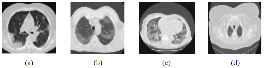
Outcomes of the NSST with Bilateral filter [25].
Outcomes of method noise-based DnCNN [26].

Outcomes of NSST with bayes shrinkage thresholding [27].
Outcomes of NSST with Wiener filter and SURELET [28].
Outcomes of tetrolet transform [29].
Outcomes of the proposed method.
The experimental outcomes of NSST with bilateral filter , as depicted in Fig. (10), show better denoising of CT images [25]. However, as the noise levels escalate, it loses its ability to preserve image detail features in higher noise regions. The findings of the proposed approach, as depicted in Fig. (15), state that the method achieves the highest PSNR values at different noise levels in images (CT1, CT2, CT3, and CT4). This means that the noise is effectively suppressed while edge details are preserved, enhancing the overall quality of the CT image. It was observed that, when compared to other methods, the low ED values at lower noise intensity levels significantly increase with rising noise. The lower ED values denote better denoising performance. The proposed method shows consistent ED values, depicting balanced denoising performance with stable accuracy across various noise levels for CT1 to CT4 images. The FSIM values are closer to 1, which denotes the optimal image feature preser -vation. The method noise-based CNN and the Tetrolet Transform perform well; however, their FSIM values decrease more significantly than those of the proposed approach under higher noise conditions. The proposed method’s SSIM values are closer to 0.999 [26, 29], indicating its effective preservation of essential structural details. The proposed approach consistently achieves the highest PSNR, SSIM, ED, FSIM and RMSE values over all CT images and different noise intensities, showing superior denoising performance and effectively preserving the edges and structural features. This highlights the proposed approach as the most resilient and reliable choice for CT image noise suppression among all the methods.
The experimental results of method noise-based CNN are shown in Fig (11) [26]. The PSNR, SSIM, ED, FSIM, and RMSE demonstrate moderate noise mitigation and feature retention but often fail to preserve edges at higher noise levels and observed promising results in the experimental outcome when compared with different noise levels. For example, The PSNR values drop from 28.19 dB to 16.35 dB (σ = 5-20), while the SSIM value decreases from 0.9054 to 0.7766 at higher noise levels, indicating challenges in edge preservation under severe noise conditions. Additionally, ED and RMSE exhibit moderate denoising performance. However, the FSIM value remains close to 1 across all CT images, demonstrating effective feature preservation. Regions with higher image details exhibit over-smoothing, causing a diminution of intricate details. The denoising results of NSST with Bayes shrinkage are displayed in Fig (12) [27]. In comparison with the proposed method, all (CT1, CT2, CT3, and CT4) images exhibit moderate denoising performance and edge preservation.
The visual outcomes of NSST with Wiener filter and SURELET are shown in Fig. (13) [28]. CT images with lower noise levels exhibit moderate denoising performance. For example, in the CT4 image, PSNR-26.85, SSIM-0.9089, ED-0.3100, and FSIM-0.9825 at σ = 5 and RMSE indicate lower noise mitigation and maintenance of edge characteristics in CT images as the noise increases. The experimental visual denoising outcomes of the Tetrolet transform, as depicted in Fig. (14), effectively perform noise minimization and edge preservation [29]. The denoising method shows competitive results at lower noise levels, achieving a PSNR value of 37.74 dB for the CT4 image, which is very close to the proposed method’s PSNR value of 41.05. In some cases, the Tetrolet Transform is less effective at higher noise intensities, resulting in limited noise suppression. Notably, in CT1 at a noise intensity of σ=20, the SSIM, ED, FSIM, and RMSE metrics indicate a significant improvement in CT image quality [29]. However, while this method preserves the overall texture of the image, it fails to adequately retain sharp image details, such as edges, as noise levels increase. The outcomes of the proposed method are shown in Fig. (15). The suggested method effectively leverages worthy features of both shearlet transform with the BayesShrink rule and guided filtering. It is clear that the noise is effectively suppressed, while edges and corners are well preserved for local details. Additionally, the smoothness over uniform regions is maintained. The proposed method significantly enhances the high-frequency components, and the BayesShrink rule is used to calculate the optimal threshold value for effective noise suppression and guided filtering on low-frequency components to preserve edges, thereby improving overall imaging quality.
The denoised CT3 image with an annotated line segment is depicted in Fig (16). The intensity profiles help to visualize abrupt variations in intensity values, indicating the image’s edge details. The intensity profiles of the noise-free image, noisy-image, various denoising methods, and the proposed technique are shown in Fig (17).
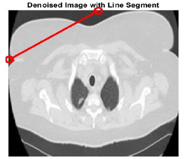
The linear segment serves to represent the intensity profile of the CT3 image and existing denoising techniques.
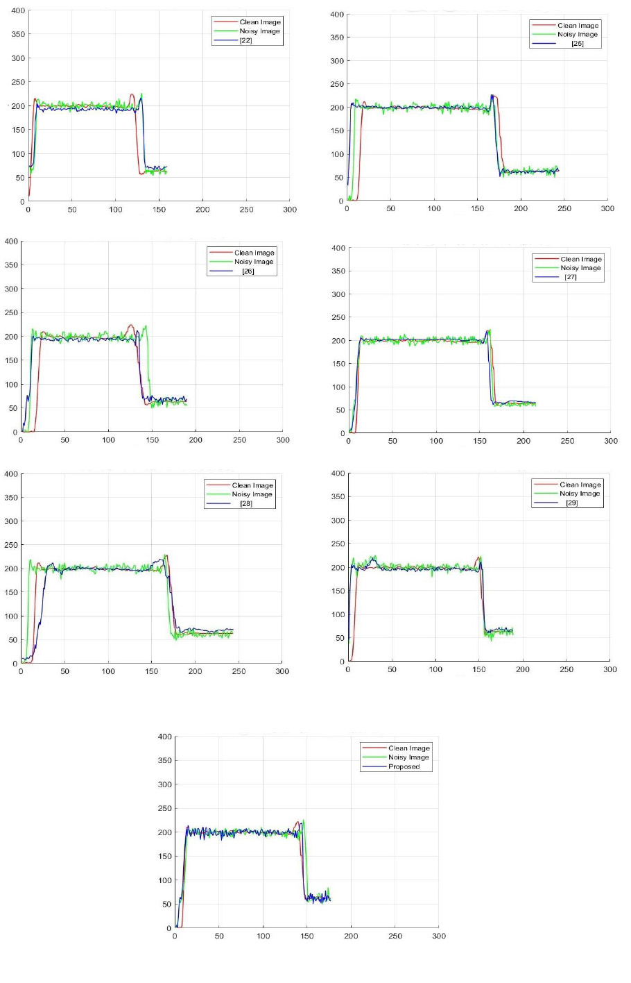
Intensity profiles of the clean image, noisy image, various denoising methods, and the proposed method. The intensity profiles are used to perform an in-depth analysis for addressing variations in pixel-intensity values with specific lines in clean images, noisy images at noise variance 10, and filtered-image. The comparison of noisy and denoised image’s intensity profile can analyze the noise level within the image and the efficacy of different denoising algorithms. The intensity profile of the ground truth image is indicated in red color, and it preserves a smooth profile in regions, and steep transitions represent edges in the image. The noisy image intensity profile is represented in green color. The noise generally introduces fluctuations in the intensity profile and shows minor irregular deviations, but noisy image signal follows the clean image but additional variability.
The denoised CT image is shown in blue color. Denoised images often follow clean images very closely, indicating that the denoising method effectively suppresses noise while preserving textures and edges of CT images. The proposed method intensity profile shows that the new denoising method successfully suppresses noise or distortion in the noisy CT image. The denoised images align well with the intensity profile of the clean CT image, indicating effective preservation of both smooth regions and edge details. This demonstrates that the proposed method outperforms existing filtering techniques in terms of noise suppression and edge preservation.
CONCLUSION
In this study, the new hybrid method introduced for CT image noise reduction and edge preservation merges Nonsubsampled shearlet transform with Guided filtering and BayesShrink thresholding. Subsequently, it integrates the result of the denoised image of the NSST framework and the application of NSST on residuals to reconstruct the final denoised image. The proposed framework effectively utilizes the strengths of NSST to capture multidirectional features and preserve fine image details, guided filtering’s capability for structural enhancement, and BayesShrink’s efficacy for noise suppression and reapplies NSST on residuals for enhanced denoising effect to elevate overall imaging quality and clarity. The comprehensive effectiveness of the proposed approach is examined and evaluated against the existing methods, in which findings show that the novel method yields improved visual outcomes in conjunction with performance measures (PSNR, SSIM, ED, FSIM and RMSE). The intensity profiles of the original image, noisy image, and denoised image were analyzed, along with additional approaches, and it was found that the proposed method achieves superior results. Therefore, it can be concluded that the proposed method effectively performs noise suppression and edge preservation, significantly improving the overall quality of CT imaging.
Future work for this study to improve the applicability of the novel proposed method in various imaging modalities like MRI and PET scans ought to be investigated to evaluate its adaptability in different diagnostic perspectives. Additionally, testing the proposed approach on diverse datasets and various noise intensity levels and scanner types would confirm its reliability and practicality.
AUTHORS’ CONTRIBUTIONS
It is hereby acknowledged that all authors have accepted responsibility for the manuscript’s content and consented to its submission. They have meticulously reviewed all results and unanimously approved the final version of the manuscript.
LIST OF ABBREVIATIONS
| PSNR | = Peak Signal-to-Noise Ratio |
| SSIM | = Structural Similarity Index Measure |
| ED | = Entropy Difference |
| FSIM | = Feature Similarity Index Measure |
| RMSE | = Root Mean Squared Error |
AVAILABILITY OF DATA AND MATERIALS
The data and supportive information are available within the article.
CONFLICT OF INTEREST
Dr. Vinayakumar Ravi is the Associate Editorial Board Member of The Open Bioinformatics Journal.
ACKNOWLEDGEMENTS
Declared None.