Advanced Machine Learning Techniques for Prognostic Analysis in Breast Cancer
Authors Info & Affiliations
Abstract
Aims
The aim of this research is mainly to use machine learning methods for forecasting significant characteristics related to breast cancer using the data to facilitate diagnosis and treatment accordingly. Such factors include the progesterone receptor status (PR+), a biomarker that helps in the understanding of the hormone receptor status of breast cancer cells, and PR status has specific prognostic value for the effectiveness of hormone therapies. Also, in the study, it is essential to predict a tumor stage, which is one of the more significant factors to determine cancer progression and treatment plan. Another focus is the prediction of the oncotree code, a hierarchical taxonomy that gives even more information about the type of breast cancer and presents the possibility of individually tailored treatments. To achieve these objectives, this study uses sophisticated classification and regression algorithms like Support Vector Machine (SVM), Random Forest and Logistic Regression. These models are implemented on the METABRIC dataset, a large-scale genomic and clinical model, to capture trends and generate precise forecasts to advance knowledge of breast cancer traits and enhance patient care.
Background
Breast cancer is the most prevalent type of cancer among women, originating in the cells of breast tissue and potentially spreading to other parts of the body, damaging surrounding tissues. Significant advancements in breast cancer research, increased funding, and heightened awareness have greatly improved early diagnosis and treatment, contributing to higher survival rates and reduced fatalities.
Objective
This research proposes the following objectives: The main objective of the study is to leverage the analysis of the METABRIC dataset to improve the prospects of personalized medicine in breast cancer diagnosis and treatment planning. Due to the availability of genomic and clinical data on METABRIC, this study aims to identify important characteristics and biomarkers in the development of tailored therapy. This work’s investigation objectives include PR+ status, tumor stage and oncotree code-defined cancer subtypes. Applying machine learning methods, such as SVM, Random Forest, and Logistic Regression, this research intends to find significant associations and establish a premise for enhancing patient prognosis and the accuracy of cancer therapy.
Methods
The METABRIC data set is used in the analysis to identify fundamental factors, including the progesterone receptor status, cancer stage and cancer type (oncotree code). This is done with the help of such machine learning algorithms as SVM, Random Forest, Logistic Regression that allow for correct modeling and deriving insights of these clinical parameters.
Results
In the proposed breast cancer classification work, higher accuracy was observed from several classifiers as per the machine learning classifiers used in the project. Among the classifiers, the classical quadratic classifier known as the Support Vector Machine (SVM) with a radial basis function (RBF) leading to a high accuracy of 99.79% when the regularization parameter (C) is at 0.001, demonstrates the effectiveness of the classifier compared to others in capturing Non-Linear patterns within the data set. The linear SVM was also very effective, achieving an accuracy of 97.93% and also demonstrating the ability to classify the data with simpler decision boundaries. Likewise, the Random Forest classifier, having high accuracy and an ensemble-based approach, expects much high strength, especially in handling the complex data and got the accuracy of 97.59%, which again proved this strength of the Random Forest classifier. However, the Logistic Regression, a simpler linear model, gave a slightly lower accuracy of 89.45%, maybe because this model does not have the ability to capture nonlinear relationships. This study also emphasizes the importance of choosing the right classifiers and setting hyperparameters that will fit the characteristics of this type of database to obtain the best performance of the classifiers. The study successfully leverages the data from the METABRIC dataset, demonstrating the effectiveness of different machine-learning models in predicting these key cancer-related factors.
Conclusion
This research contributes to the field of personalized medicine by providing objective findings on breast cancer detection and therapy. It will use the most advanced machine learning methods and the rich METABRIC data to improve the prediction of key diagnostic parameters and factors, including hormone receptor status, tumor stage and cancer subtype. These enhancements in predictive precision enable the examination of the malignant neoplasms at an earlier stage and help to design individualized treatment regimens that might be closely related to the general clinical phenotypes of the patient. Thus, this research can contribute to the delivery of better patient care through better therapeutic targets and approaches that are specific to the breast cancer context.
1. INTRODUCTION
Breast cancer is the most common invasive cancer in females besides skin cancer illness. Cancer of this type develops when cells in the breast start to divide in an uncontrolled manner and form a lump that can be felt with the hand. As with most cancers, breast cancer mainly occurs in women, although men can also be diagnosed with this disease. The disease has symptoms, and these come in different types including Ductal Carcinoma and Lobular Carcinoma. Ductal Carcinoma begins in the cells forming the lining of ducts that carry milk from the breast glands to the nipple. This is a common type of cancer and is more often diagnosed early because it is found near the milk ducts. On the other hand, Lobular Carcinoma starts in the lobules, which is a gland that secretes milk. This type is a little rare but can be hard to diagnose early because it originates far down in the breast tissue [1]. Breast cancer is a health problem of considerable magnitude throughout the world. In 2018, it was estimated that over 600,000 deaths from breast cancer occurred worldwide, affecting both women and men. The global burden of this disease underscores the importance of awareness, early detection, and advancements in treatment strategies to reduce mortality rates. Fig. (1) is a combined anatomical and epidemiological representation that can serve as a helpful tool in gaining an increased understanding of the field of breast cancer. A cut out on the breast structure is provided and the main parts of the breast: lobules, ducts, and fatty tissue are pointed out since they are all involved in cancer. In addition to this, the statistics on types of international breast cancer cases provide information on the diseases’ popularity and the existence of this problem in different countries and among different age groups. Altogether, these visuals highlight calling for more research to help minimize the burden of breast cancer in the world, which is mentioned in source [2].
Fig. (2) highlights the global distribution of breast cancer occurrences, illustrating the widespread impact of this disease across different regions. The figure provides a visual representation of how breast cancer affects populations around the world, emphasizing the varying incidence rates in different countries and continents. This geographic variation is influenced by several factors, including genetic predisposition, lifestyle, environmental influences, and the availability of healthcare services. This type of data could help researchers and healthcare professionals gain a small glimpse at how breast cancer is affecting the globe, where the dangers live, and how to go about tackling the breast cancer problem. Such exhaustive analysis of breast cancer points to the need for international collaboration and resource mobilization required in the fight against this disease.
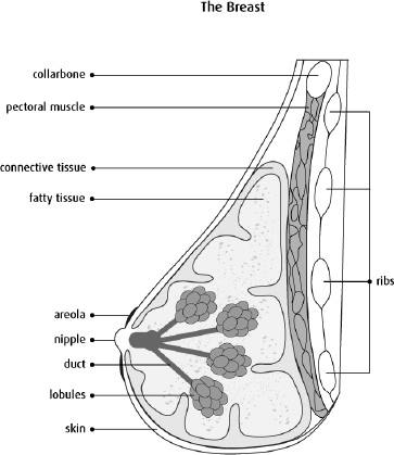
Structure of a breast [1].
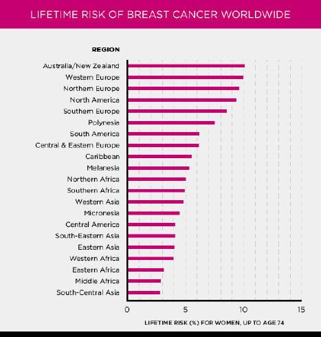
Cases of occurrence of breast cancer world wide [2].
1.1. Symptoms of Breast Cancer
The signs and symptoms of the early stage of breast cancer should be detected so that early treatment is possible. The following symptoms are commonly associated with breast cancer and should not be ignored:
1.1.1. Lump or Hard Knot
Swelling of the breast or formation of a lump or hard knot in the breast or underarm is the sign commonly attributed to breast cancer.
1.1.2. Swelling or Redness
Just enlargement of the skin on the breast area, redness or darkening ultimately could be as a result of a certain disease.
1.1.3. Changes in Breast Size or Shape
The changes in size and shape of the breast should not be any normal occurrences and should be investigated.
1.1.4. Itchy Sensation or Rash on the Nipple
Other symptoms which may be symptoms of breast cancer include itching and harsh or ridged feeling around the nipple or the presence of a rash on the nipples.
1.1.5. Nipple Discharge
Any gush from the nipple, especially that containing blood, should cause alarm.
1.1.6. Localized Breast Pain
Feelings of pain at any location in the breast are also a symptom that requires attention.
1.1.7. Dimpling of Breast Skin
Rounding or skin dimpling, which may make the skin look like the outer skin of an orange is another sign requiring attention.
1.1.8. Inward Pulling of Nipple or Skin
All drawing in or retracting of the nipple or breast skin is a symptom that requires one to see a doctor.
However, it should also be remembered that not all of these are symptoms of breast cancer, but it is advisable to seek medical attention if experiencing them. It is, therefore, important to remain fully aware of these signs and symptoms so that the conditions can be detected and treated early.
1.2. Causes of Breast Cancer
Much as numerous studies have been conducted on the factors that cause breast cancer, its causation is still unknown and doctors and scientists continue researching. However, studies have identified several key factors that are believed to increase the risk of developing breast cancer:
1.2.1. Family History
When a woman has relatives with breast cancer, especially mothers or sisters, her risk is considered significantly high.
1.2.2. Age
Age is another factor that influences susceptibility to breast cancer in women and as with most cancers, the older the woman, the higher her risk.
1.2.3. Alcohol Consumption
Intake of alcohol has been found to increase the tendency to develop breast cancer disease.
1.2.4. Use of Birth Control Pills
Long-term use of contraceptives may actually slightly increase the risk of breast cancer in women.
1.2.5. Breast Density
Women with glandular and fibrous breast tissue are more susceptible to developing breast cancer since the glandular tissue obscures the tumour in mammograms.
1.2.6. Prolactin Levels
The study found that women with high levels of prolactin, the hormone that causes the breasts to grow and produce milk during breastfeeding, could be at a higher risk of developing breast cancer.
1.2.7. Radiation Exposure
Breast cancer may also occur from radiation, especially for women who were exposed to radiation at young ages up to the age of 30.
1.2.8. Age at First Childbirth
Women who gave birth to their first child at a more advanced age may be at greater risk than those who began childbearing at an early age.
1.2.9. Insulin-like Growth Factor 1 (IGF-1)
IGF-1 is a hormone that is important in body growth and development. It has been detected that the concentration of IGF-1 in the bloodstream increases the causal risk of breast cancer. However, this relationship indicates that high IGF-1 levels can promote the development of new breast cancer cells.
1.2.10. Inherited Gene Mutations
BRCA1 and BRCA2 are known genes that increase susceptibility to breast cancer through mutations. They can be passed from one generation to another and most of them will result in the early emergence of the disease. However, other gene mutations that affect cancer risk are also present, like the TP53 or PALB2 genes, at a significantly lower prevalence.
These factors, although cannot be termed predictors but, are taken into consideration when assessing the risks of breast cancer. Further research is still being conducted on other possibilities, as are other causes of the disease, in order to enhance the studying of the sickness and findings on favorable ways of preventing the sickness.
A case-control gene expression study across subordinate types of breast cancer has suggested that one gene heritability trait associated with the disease risks is the BRCA1 and BRCA2 genes. Some of them can be inherited, which means that such risks of developing breast cancer are very high.
In women aged 70 years and older, the likelihood of getting breast cancer if one has a BRCA1 gene mutation is between 55%- 65%. Likewise, women with BRCA2 gene mutation have approximately a 45% chance of getting this disease. Such statistics indicate how genetics are a central predisposing factor towards breast cancer, hence the need for genetic tests and counseling in affected families. Awareness of such risks enables the prescription of more relevant and effective measures of prevention, early detection and subsequent treatment.
1.3. Diagnosis and Treatment
Breast Cancer can be diagnosed through Mammograms, Breast MRI, and Biopsies. The course of treatment usually depends on the severity of the cancer cells spread into the body, the size of the tumour, the stage of cancer, and of course, the medical history of a patient [2]. Following are the different ways doctors could treat breast cancer:
- Surgery
- Radiation therapy
- Chemotherapy
- Hormone therapy
- HER2-targeted therapy
- Oral cancer drugs
Every treatment has its own side effects, mostly including fatigue, loss of appetite, nausea, constipation or diarrhoea, hair loss, mouth sores, and skin and nail problems. For this disease to be caught as early as possible poses immense importance because the earlier the diagnosis, the more chances of survival there are for the patient and the course of treatment is much less painful.
2. METHOD
The structure of the research is organized into the following sections: Section 2 presents a brief discussion of literature works related to this research, Section 3 explains the method presented in this study and gives information about the data set used in this study, Section 4 presents an evaluation of the classification performance achieved by the proposed method and Section 5 provides the conclusion of this study with findings revealed from this study.
2.1. Related Works
Gonca Buyrukoglu et al. [3] explained ensemble learning techniques like random survival forest and conditional inference forest outperform the Cox proportional hazards model for prognostic analysis in breast cancer survival prediction. Olukayode Felix Ayepeku et al. [4] explore various machine learning models like Logistic Regression, Decision Tree, and XGBoost for breast cancer prediction, emphasizing their effectiveness in prognostic analysis. Karthikeya Mallelli et al. [5] explained different Machine learning techniques, including CNNs, LSTM, and RNN, are utilized for prognostic analysis in breast cancer, aiding in accurate classification and prediction tasks based on gene expression data. P. Bhaskar et al. [6] explore various machine learning models like random forests, logistic regression, and deep learning neural networks for predicting breast cancer outcomes, emphasizing early detection's crucial role. Julian Paul et al. [7] explained Deep learning model DiaDeepBreastPRS predicts 5-year survival in breast cancer patients using histopathology images, showing potential for advanced prognostic analysis in breast cancer with high accuracy. Chirayou Bista et al. [8] explained the Breast Cancer Prediction System utilizes Random Forest, SVM, and Gradient Boosting Ensemble for accurate prognostic analysis, enhancing early detection and prognosis in breast cancer. Srikanth Gadamsetty et al. [9] research integrates deep learning and machine learning to predict breast cancer subtypes and identify key mutations, showcasing advanced techniques for prognostic analysis in breast cancer. S Balasubramaniam et al. [10] Ensemble learning, particularly XGBoost, proved superior in predicting breast cancer incidence, showcasing advanced machine learning techniques for prognostic analysis in breast cancer. Jordan, Alzu’bi et al. [11] applied machine learning techniques with the aim of enhancing the extraction of critical information from computerized health records at King Abdullah University Hospital. Their work involved developing a natural language processing system that facilitated the creation of a specialized medical dictionary focused on breast cancer, thanks to the integration of these advanced elements. Rana et al. [12], machine learning techniques were employed to focus on both the diagnosis of breast cancer and the prediction of its recurrence. The results provided a detailed examination of four various machine learning algorithms and compared their performance. The outcome also showed that random forest was particularly suitable for the highest accuracy in the predictive analysis and SVM for an extremely satisfactory success rating in predicting the malignant cases and separating those cases that recurred with those thatdid not. The current study focuses on the application of machine learning in the automated diagnosis of breast cancer where early detection is shown to significantly determine the results of treatment.
The researchers undertook a research the main aim of which was to develop ensemble machine learning algorithms to forecast breast cancer [13]. The research conducted by them was on the”Breast Cancer database,” where they compared different risk factors like family history of cancer, lack of physical activity, stress, and breast size for the diseases. In this work, the authors sought to improve their ensemble models by including these factors to make a better prediction of breast cancer risk. In another study, the predictors of tumor recurrence estimated by MRI-based radiomics features with Oncotype DX-tested invasive ER+/HER2- breast cancer patients were evaluated [14]. The analysis involved a group of a total of 62 patients. To estimate the prediction of the recurrence risk, the radiomics feature vectors were derived for both tumor and peritumoral tissue. In a rather related study [15], the authors employed machine learning methods to antecedent disease relapse in post-surgery breast cancer patients despite optimal treatments. They also used specifics of clinical data that were extracted from 2-deoxy-2-(18F)-fluoro-d-glucose positron emission tomography ((18F)-FDG-PET) scans and the radiomic features of the input images to improve the model’s performance. Recent works [16-19] have highlighted the contribution of the machine learning models in invasive breast cancer diagnosis as having enormous potential for enhancing diagnostic accuracy and early detection. A logistic regression analysis has proven very effective attaining 97% accuracy precision rates of 98% for the benign case and 97% for the malignant case. RF models also proved to have good performances; one paper showed an accuracy of 98.25% in classifying breast biopsy samples classification, and another paper showed 96% accuracy. However, there is a relatively less consistent accuracy attained from SVM and DT models while the models based on Logistic Regression (LR) and Random Forest (RF) have given better results. Additionally, by combining machine learning with imaging technologies like mammograms and MRI, the detection abilities have improved. However, still, issues such as data quality and model interpretability are hurdles to the clinical use of such models.
2.2. Proposed System
The identification of a breast cancer detection system is presented in the form of a flowchart in Fig. (3), which provides an accurate and coherent breakdown of the methodology used. On the flowchart, all the steps can be seen, starting from the preprocessing of data and feature extraction up to the point of applying machine learning for classification or prediction. They underline its sequential character, the input of data, the further training and validation of the model, and, finally, the obtaining of diagnostic data. As a result, with the help of the figure, it is possible to provide the reader with various advantages: making the approach transparent and visually divided into steps, as well as stressing the specific nature of the offered detection and diagnosis system.
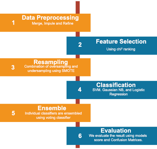
Flowchart of proposed breast cancer detection system.
The process begins with the data collection phase, where relevant patient information and medical imaging data, such as mammograms, are gathered. This data forms the foundation upon which subsequent analyses are conducted. Next, the preprocessing stage ensures that the collected data is cleaned and prepared for analysis. This step may involve removing noise from images, normalizing data, and extracting essential features that are crucial for accurate diagnosis. Following preprocessing, the feature extraction step isolates key attributes from the data that are indicative of breast cancer. These features may include the size, shape, and texture of tumors, as well as other biomarkers that are commonly associated with malignancies.
The extracted features are then fed into a machine learning model designed for classification. This model has been trained on a vast dataset of labeled examples, enabling it to distinguish between benign and malignant cases with high accuracy. The flowchart depicts the decision-making process of the model, illustrating how it categorizes each case based on the input features. In cases where the model identifies a potential malignancy, the diagnosis step is initiated. Here, the results are carefully reviewed, and the system may generate a detailed report outlining the likelihood of breast cancer and suggest further diagnostic tests or treatments.
Finally, the output phase consolidates the findings, providing healthcare professionals with actionable insights that can guide patient care. This final step ensures that the detection system not only identifies potential cancer cases but also supports medical decision-making with clear, evidence-based recommendations.
Overall, the flowchart in Fig. (3) encapsulates the entire workflow of the breast cancer detection system, from data acquisition to final diagnosis, ensuring a structured and reliable approach to early cancer detection.
2.2.1. Dataset
Our dataset is provided by Metabric (Molecular Taxonomy of Breast Cancer International Consortium). It is a Canada-UK-based study group that aims to classify breast tumours into further categories, on the basis of which doctors can determine the course of treatment [3]. The dataset consists of two files. One file containing the gene information of about 24,368 genes and the other file containing the clinical data of the 2,173 sample patients.
2.2.2. Data Preprocessing
2.2.2.1. Data Merging
We had two dataset files, one containing the gene information and the other containing clinical data of patients. Both files contained the patient ID on which we merged the two files. We faced a problem in the process of merging when it came to the gene expression dataset because it had all the patient IDs in columns rather than rows. As a solution we transposed the gene data so that all the genes (features) are in columns. After then, we finally merged the dataset using pd.merge, taking a joint on patient ID.
2.2.2.2. Data Cleaning
After we got our final dataset, we performed cleaning. In this step, we dropped all the redundant columns containing the same values, which do not contribute to prediction. For example, we dropped Metaplastic breast cancer (MBC) because it only contained one value,”Breast Cancer”.
2.2.2.3. Data Imputing
Before transforming the data, the presence of missing values and NaN entries exposed to them by replacing them with the mean of that column, respectively. This way, the dataset remains structurally sound for analysis and the data that would have been missing are also avoided and will not introduce a bias in the results. Doing so means that while missing values are replaced with means, the overall spread of a given dataset is retained, thereby not affecting the performance of machine learning algorithms by feeding them with data they are not equipped to analyze. This step of preprocessing is important for preserving the results’ coefficients and the credibility of the predictions.
2.3. Feature Selection
We performed feature selection because we had about 24,368 gene features. So, we removed irrelevant and redundant features from our dataset which resulted in better performance of the classifier. We use Chi-Square for feature selection for Classifying Tumor Stage, and oncotree code. Scikit learn library provides us sklearn.feature selection.chi2(X, y) function to perform feature selection. It basically works by selecting the best features based on the values of the chi-squared statistic test. The chi-squared test basically indicates the dependence of the variables, so we select the features with the highest scores and remove all the features that seem to be independent from the class and thus do not contribute to classification. We first performed classification by selecting 2000 features and then later by 5000 features, which resulted in giving much better accuracies.
2.4. Sampling Data
Before diving into the Classification, we studied our data to check if it was balanced. For each label, we found out the number of rows. For oncotree code, the following are the number of rows
in each class:
- BREAST - 17 rows
- IDC - 1499 rows
- ILC - 142 rows
- IMMC - 22 rows
- MDLC - 207 rows
For the Tumor Stage, we have the following:
- Stage 0 - 4 rows
- Stage 1 - 474 rows
- Stage 2 - 800 rows
- Stage 3 - 115 rows
- Stage 4 - 9 rows
For PR Status, we have the following:
- Positive - 1009 rows
- Negative - 894 rows
For our dataset, the dimensionality is high and since the classes are highly imbalanced in the oncotree code and tumor stage, the accuracy of our classifier will be reduced. There are four ways to deal with this problem:
(1) Synthesise of new minority class instances
(2) Over-sampling of minority class
(3) Under-sampling of majority class
(4) Tweak the cost function, such as misclassifying minority class instances has more penalty than majority class instances.
To avoid this problem, we resampled our data using the package - SMOTE.
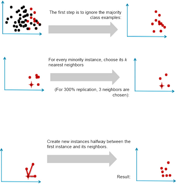
Generating new minority samples using SMOTE.
SMOTE stands for Synthetic Minority Oversampling Technique. It is one of the many available techniques to tackle the problem of class imbalance. SMOTE synthesizes new minority instances between real minority instances [4]. This implementation of SMOTE makes the number of minority instances the same as a number of majority instances. It applies the K-NN algorithm to join the existing instances and creates a synthetic sample in that space. The algorithm takes samples of the feature space for each target class and generates new examples that satisfy the feature space of its neighbors (Fig. 4).
Fig. (5): This figure could show the class distribution for the first target variable. For example, if it is a binary classification problem, this might show an imbalance where one class has significantly more instances than the other.
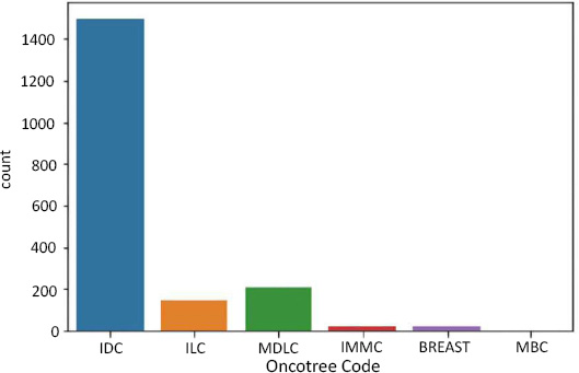
Data imbalance in oncotree code as target.
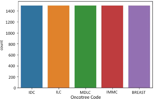
Data resampling for oncotree code.
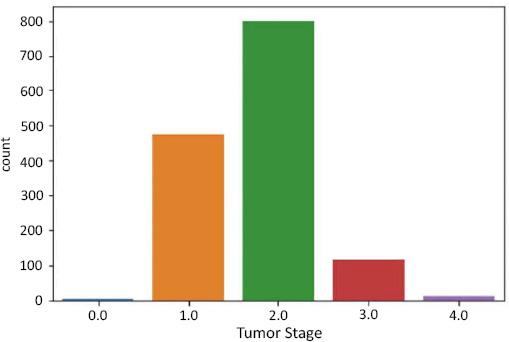
Data imbalance in tumor stage as target.
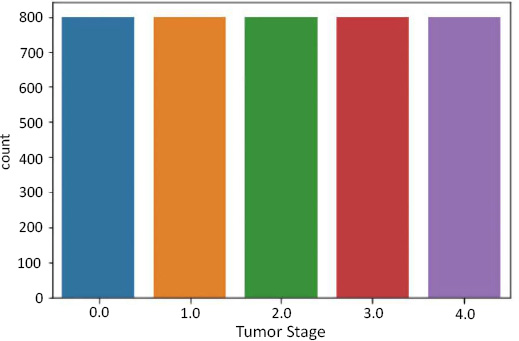
Data resampling for tumor stage.
Fig. (6): After applying SMOTE to the first target variable, this figure illustrates how the class distribution has changed. SMOTE works by generating synthetic samples for the minority class, thereby balancing the number of instances across classes.
Fig. (7): This figure might depict the class distribution for a second target variable. If there are more than two classes, this could show how some classes are underrepresented compared to others.
Fig. (8): For the second target variable, this figure would show how the class distribution has been adjusted post-SMOTE. Ideally, the previously underrepresented classes should now have a number of instances closer to the majority classes.
Fig. (9): Similarly, this figure would display the class distribution for the third target variable, highlighting any imbalances that might affect model performance.
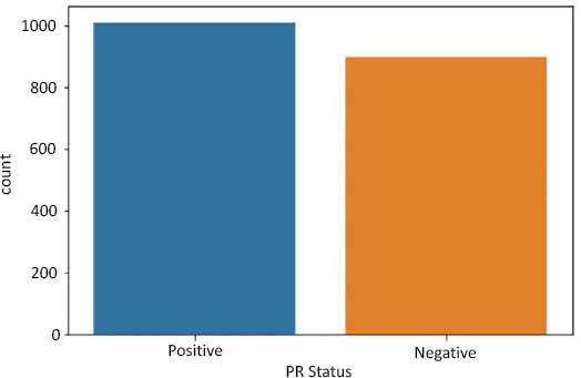
Data imbalance in PR status as a target.
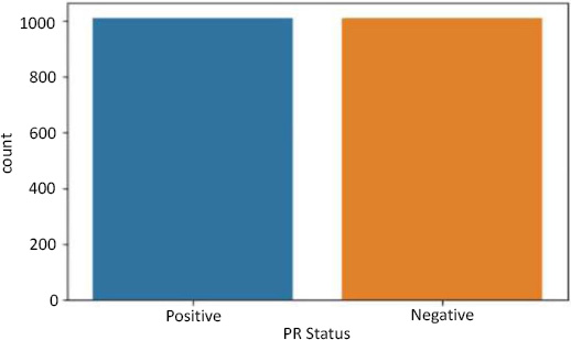
Data resampling for PR status.
Fig. (10): This figure would represent the class distribution for the third target variable after SMOTE application. The goal is to achieve a more balanced distribution that can help improve the performance of machine learning models.
The purpose of these figures is to visually confirm that SMOTE has effectively balanced the class distributions and to provide a comparison between the before and after states of class distributions.
In summary, Figs. (5, 7, and 9) reveal the initial class imbalances, while Figs. (6, 8, and 10) show the improvements made through SMOTE resampling, helping to ensure that the dataset is more balanced for training your models.
2.5. Classification
After feature selection and resampling, we finalized a version of the dataset ready for classification. We have used four different classification techniques i.e., Logistic Regression, Support Vector Machines (SVM) with Linear Kernel, Support Vector Machines (SVM) with RBF Kernel, and Random Forest. The detailed working of each algorithm is explained below:
2.5.1. Logistic Regression
Logistic Regression is the most preferable technique to use when our target variables are categorical. There are three types of logistic regression:
2.5.1.1. Binary Logistic Regression
The class labels have only two possible outcomes. Example: PR status has only two values, positive and negative.
2.5.1.2. Multinomial Logistic Regression
The class labels have three or more possible outcomes. Example: oncotree code has about six possible values which are IDC, ILC, MDLC, IMMC, BREAST, and MBC.
2.5.1.3. Ordinal Logistic Regression
The class labels have three or more categories, but they are in order. Example: tumor stage: 0,1,2,3, and 4. We used the scikit library’s function sklearn.linear model.logistic regression for predictive analysis and chose the value ‘auto’ for the argument ’multiclass’, which decides which type of logistic regression to apply. Logistic regression works by predicting the probability of an occurrence of a target variable by fitting the data to a logit (sigmoid) function shown in Eq. (1) [10].
 |
(1) |
2.6. Support Vector Machine (SVM)
Support Vector Machine is a supervised machine learning algorithm as shown in Fig. (11). Support Vector Machine (SVM) (from [9]) create a hyperplane that successfully classifies all its data points in an n-dimensional feature space where n is the number of features. As shown in Fig. (11), support vectors are the data points closest to the hyperplane. SVM draws a hyperplane in such a way that maximizes the margin, meaning the distance between points that are closest to the other class points [11].
Support Vector Machines are very powerful when it comes to classification. As we have studied, SVM draws a linear hyperplane between the classes, but what if the classes aren’t linearly separable? SVM uses a trick called the Kernel trick. These functions map the data points to higher dimensions where the problem is linearly separable and SVM can draw a hyperplane correctly classifying our target variables [12]. We used the RBF kernel for our problem as it maps data to infinite higher dimensions, giving us a very good accuracy that will be explained in the next section. RBF kernel function is shown in Eq. (2).
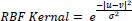 |
(2) |
2.7. Random Forest
Random Forest is a powerful yet very flexible machine learning technique. It is basically a large group of relatively uncorrelated decision trees that are merged together to get a more accurate result. The key reason behind the good accuracy is the uncorrelation between the trees; when one tree is wrong, the others might be right, so their combined effect is always right. Random Forest usually produces the correct result even without a hyper-tuning parameter, as shown in Fig. (12). The higher the number of uncorrelated trees in the model, the better the accuracy [13].
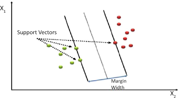
Support vector machine (SVM).
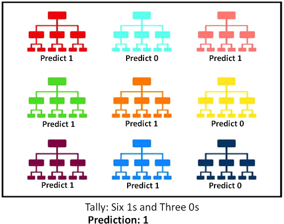
Random forest.
2.8. Ensemble
In Machine Learning, ensemble learning uses multiple learning algorithms to obtain better predictive performances than those that could be obtained from any of its constituting learning algorithms [6]. To avoid overfitting in a single classifier, we have used ensemble learning. In our project, we use Voting Classifier, an ensemble learning technique in sklearn. The idea behind the Voting Classifier is to combine conceptually different machine learning classifiers and use a majority vote or the average predicted probabilities (soft vote) to predict the class labels [7].
This model is used for equally well-performing models so that they cover their weaknesses when used together in a voting ensemble. We have used a hard voting strategy in the Voting Classifier and found the average accuracy. Ensemble allows us to have a much more flexible model to exist amongst all the other alternatives.
2.9. Evaluation
After performing classification and obtaining the predicted labels, we evaluate the models using the score attribute of sklearn models, which returns the mean accuracy on the given test labels [8].
For multi-class prediction, which is the case in tumor stage and oncotree code, just knowing the mean accuracy is a harsh metric since we require, for each sample, each label to be predicted correctly. Therefore, we also print the confusion matrix.
Confusion Matrix is generally used in a binary classification, but for multi-class classification, we treat each label as a one vs all case, and get a confusion matrix for each label. We used a multilabel confusion matrix package from sklearn. We defined our output label in the parameter and got the confusion matrices in that particular order. The confusion matrices for each target variable are discussed in detail in Section 5 of this paper.
2.10. Visualization using Dimensionality Reduction
Data Visualization is required in order to view the number of possible clusters and identify different patterns in data. Our dataset has about 24,368 features, so how do we visualize our data? Fig. (13). PCA on oncotree code Before Resampling Fig. (14). PCA on oncotree code After Resampling To solve this problem, we use Principal Component Analysis (PCA). PCA detects the correlation between variables. In simple words, PCA finds the direction (eigenvector) for which the variance is maximum. This is named as the First Component. For our purpose, we choose 3 components, as we can visualize our data in at most 3 dimensions. Therefore, as a result, we get 3 new dimensions with the highest variances. Figs. (15-18).
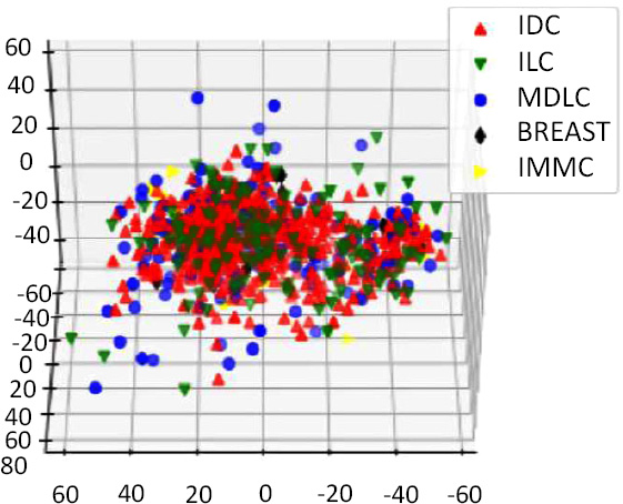
PCA on oncotree code before resampling.
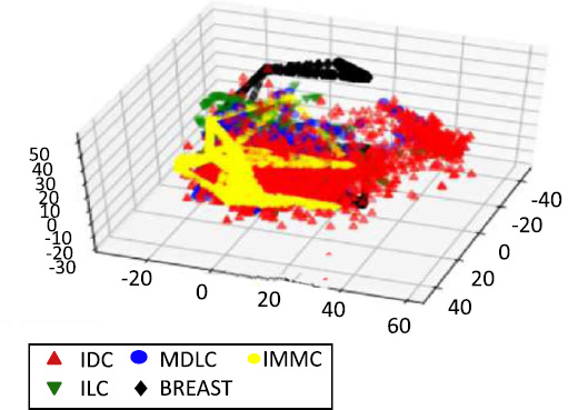
PCA on oncotree code after resampling.
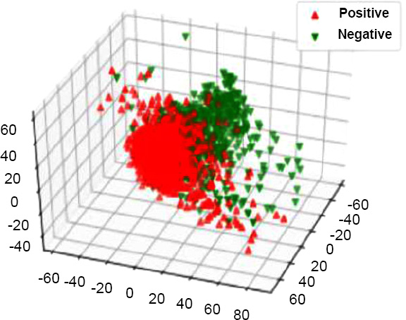
PCA on PR status before resampling.
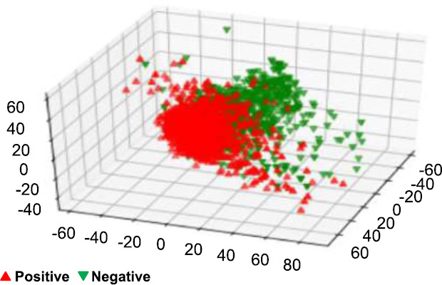
PCA on PR status after resampling.
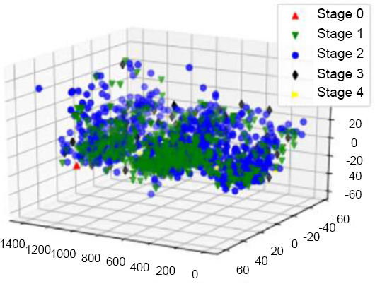
PCA on tumor stage before resampling.
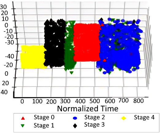
PCA on tumor stage after resampling.
The down-sampling formula, which is _c1 > _c2 > _c3, was used in the dimensionality reduction process to reduce the dataset while capturing major features. After this reduction, the dataset was visualized to observe patterns by labeling points based on the predicted values for the target variables: Tumor Stage, oncotree code, and PR Status are included among them.
The apt visualizations of a reduced set of data for each target variable before SMOTE resampling are shown in Figs. (13, 15 and 17). Such plots show the spread and density of the point cloud to bring out cases where there can be skewed distribution.
In Figs. (14, 16 and 18), we have the visualization after performing SMOTE resampling. The sampling technique also corrects the problem of class imbalance in a dataset by creating more synthetic instances of minority classes. The distinct patterns also depict a far superior balance as well as compact and well-separated clusters in comparison to the initial post-SMOTE representations, which in turn shall lead to better training of the machine learning algorithms and concrete and reliable predictions for each of the target variables.
3. RESULTS AND DISCUSSION
3.1. Individual Classifiers
After finishing classification with SVM using Linear and RBF kernel, Logistic Regression and Random Forest. We performed classification using 2000 and 5000 K-Best Features. Upon observing the results, we decided to consider 5000 features for our final evaluation as they gave all models almost similar. We have used RBF kernel with gamma 0.00045 which achieved 88.86% accuracy. We see that the RBF kernel on SVM gives us better accuracy than the linear kernel RBF and Logistic Regression (except in PR status, where it is equal). This is because the RBF kernel performs the kernel trick by finding the dot product of two input vectors and then calculating their projection in a higher (infinite) dimension in such a way that it becomes linearly separable in that dimension. We also see the accuracy of Random Forest is high, and in the case of PR Status, even higher; this is because Random Forest is a kind of ensemble, and as we have discussed, ensembles avoid overfitting by increasing variance and including different models. In a random forest, there are many base estimators, which are nothing but decision trees generated randomly. The final prediction of the Random Forest model is a majority vote of the individual trees.
The performance of the classifiers employed in predicting the level of cancer-related factors from the METABRIC data is given in Table 1. Support Vector Machine with linear kernel proved to be very efficient with 97.93% accuracy. When the SVM was used with RBF kernel and a tuning parameter value of 0.001, the results showed that the accuracy was 0.9979%, proving that the model was good for this particular work., a simpler model, yielded an accuracy of only 89.45%, which makes us wonder if more complicated models like SVM are better suited for this dataset. Last but not least, the Random Forest classifier identified the test data set with 97.59% accuracy and was also equally good but slightly less compared to the model with the SVM with RBF kernel. The SVM (RBF) model presented here returns the highest prediction accuracy for cancer-related classifications in the METABRIC dataset.
| Classifier | Accuracy % |
|---|---|
| SVM (linear) | 97.93 |
| SVM (rbf 0.001) | 99.79 |
| Logistic Regression | 89.45 |
| Random Forest | 97.59 |
As shown in Table 2, the METABRIC dataset and the compared classifiers exhibit the rates of accurate prediction of stages of tumor. Among the tested classifiers, the best results were observed when using a Support Vector Machine with the linear kernel (mean accuracy 89.5%); the classifier’s performance was satisfactory in terms of tumor staging. A similar trend was observed when the SVM was applied with RBF kernel and the SVM regularization parameter of 0.001; a prediction accuracy of 93.25% was achieved; this confirmed improvement in the prediction models. On the other hand, logistic regression, which is a more basic model when compared to SVM, only achieved an accuracy of 81.75%, proving that it may not have the capability to classify the stage of the tumor well enough. The Random Forest classifier, in turn, achieved 88.62% accuracy, which is a bit worse compared to the linear SVM yet also points to fairly good predictive performance. In general, the current study revealed that the reported SVM with the RBF kernel had been found to be superior when compared to all the other classifiers, as it correctly predicted the tumor stage of cancer patients.
| Classifier | Accuracy % |
|---|---|
| SVM (linear) | 89.5 |
| SVM (rbf 0.001) | 93.25 |
| Logistic Regression | 81.75 |
| Random Forest | 88.62 |
Table 3 summarises the performance of various classifiers in yielding the PR status from the METABRIC data set. The results for the model optimized with a linear kernel and a regularization of 0.0025 were an accuracy of 87.37%. A further enhancement of accuracy to 88.81% was observed when SVM was trained with RBF kernel and a fixed regularization parameter of 0.002. The lowest-level model was Logistic Regression and, interestingly, it reached the same accuracy as the model with the RBF kernel of the SVM at approximately 88.81%. The accuracy level recorded for the Random Forest classifier was slightly higher at 89.10%, implying that the out-of-bag classification of PR status was slightly better than the other random models proposed. These results mean that both SVM (RBF) and Logistic Regression models show comparable performance, while Random Forest outperforms them by providing the highest accuracy with regard to this classification task.
| Classifier | Accuracy % |
|---|---|
| SVM (linear c= 0.0025) | 87.37 |
| SVM (rbf 0.002) | 88.81 |
| Logistic Regression | 88.81 |
| Random Forest | 89.10 |
| Target Label | Accuracy % |
|---|---|
| oncotree code | 98.20 |
| Tumor Stage | 90.25 |
| PR Status | 89.60 |
3.2. Ensemble Learning
Results after combining the individual classifiers using a Voting Classifier are shown in Table 4. Table 4 also summarizes the results of the performance evaluation of the ensemble model for predicting the specified target labels from the METABRIC data set. The ensemble model attained an accuracy of 98.20% for predicting OncoTree whereas it has excellent results in classifying type of cancer. In terms of tumor stage prediction, the contribution of the ensemble model increased the accuracy by 90.25% that it better for some singular classifiers. Last, for predicting progesterone receptor (PR) status, the given ensemble model created with the help of the feature selection algorithm has 89.60% accuracy therefore, it possesses relatively high accuracy when compared with Single classifiers like RF and SVM. The results presented here underscore the possibility of enhanced classification accuracy via an ensemble learning approach to the targeted labels.
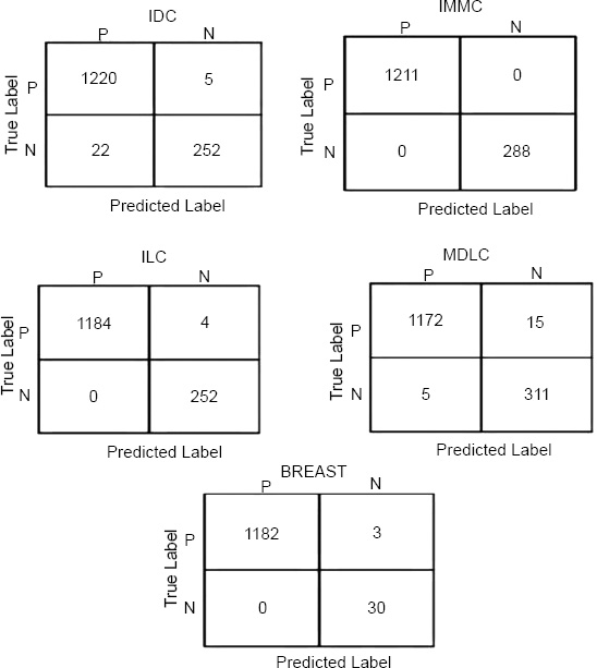
Confusion matrices for oncotree code.
As we can see, the ensemble accuracy is better than the individual classifiers. Ensemble always performs better than the individual classifiers when the individual classifiers have similar accuracy. But in the case of Tumor Stage and oncotree code, we have individual classifiers with somewhat varying accuracies. In oncotree code and Tumor Stage, we have the RBF kernel of the SVM classifier outperforming others by a considerable margin, while in PR Status, the accuracy of each model is somewhat similar; therefore the accuracy of the ensemble in PR status is higher than the individual classifiers.
Finally, we have used a confusion matrix, which is oriented to show the amount of correct and incorrect values for each class and, therefore, gives a panoramic view of the performance of our model. For multi-class classification problems, we used the multilabel confusion matrix from sklearn, which was ideal for calculating models with multiple target labels. (Figs. 19-21) illustrate the confusion matrices for the Voting Classifier ensemble–used for each of the target variables. These matrices are general in the performance of the ensemble model in predicting oncotree code, Tumor Stage, and PR Status and distinguish the true positives, false positives, true negatives and, false negatives. What needs to be emphasized here is that the confusion matrices presented below are computed for the Voting Classifier only and not for the classifiers separately. If the Reader wishes to gain deeper insight into the specifics of each classifier's decision-making, confusion matrices for all classifiers for the test set used are provided in the form of Jupyter Notebooks attached to this document. This enables the researchers to have a better interpretation of the general performance of each classifier in fulfilling the ensemble approach’s goals.
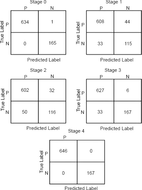
Confusion matrices for tumor stage.
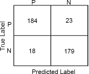
Confusion matrices for PR status.
The results have shown that our model works well when diagnosing the stages and types or cancer from the METABRIC dataset, especially in the accurate classification of Stage 4 tumor stage and IMMC OncoTree tumors, of which the model failed to misclassify a single sample. This supports the fact that this model has high accuracy and is an efficient one in categorizing these specific categories. Additionally, the model exhibited only a few misclassifications in other categories: The breast cancer achieved by GAN misclassified only 4 samples for the ILC (Invasive Lobular Carcinoma) oncotree code and 3 samples for the BREAST oncotree code cancer type. Such low misclassification rates only indicate that the model proposed here is accurate and reliable in general and is indeed accurate to some extent in classifying different stages of tumor and different types of cancers, though with some mistakes in these special cases. Finally, this performance shows that the presented model is beneficial for clinical applications in which precise cancer classification is critical.
CONCLUSION
The assessment of our breast cancer detection model has shown considerable accuracy in four classifiers used (SVM, Logistic Regression, Random Forest, and the Voting Classifier). Hence, these excises support the need for the 5,000 features (genes) chosen through feature selection where the features shown below were accurately predicted: oncotree code, Tumor Stage and PR Status. The results of these classifiers, especially the specified best classifier, the Random Forest model, with fair accuracy, argue this point by showing that these selected genes are relevant in the characterization of breast cancer. The features found here are crucial for the current advancements in breast cancer and may hold great potential for future research and treatment. Thus, we translate a huge amount of genes into a manageable number of crucial features and offer investigators and clinicians the list of promising genes for further elaborate study as potential diagnostic markers, drug targets and therapeutic strategies. In addition, with the help of the Random Forest classifier, we have identified the ten most important features, that could be considered potential biomarkers of breast cancer. This finding sets the stage for subsequent investigations of those features in other populations to confirm their reliability and of the molecular underpinnings involved to improve on the current model. Finally, we discussed the directions in which this research can be continued and improved in the future. First, it would be informative to consider using more genomic data along with other biological features than inclusion could enhance the model performance in risk prediction. The use of additional omics data (protein, metabolite, and gene expression) might provide a better understanding of the cancer mechanisms and might improve the prognosis model’s performance. However, using the proposed more sophisticated feature selection approach based on deep learning could also be beneficial for discovering better features and additional improvements to the set of features.
AUTHORS’ CONTRIBUTION
It is hereby acknowledged that all authors have accepted responsibility for the manuscript's content and consented to its submission. They have meticulously reviewed all results and unanimously approved the final version of the manuscript.
LIST OF ABBREVIATIONS
| RBF | = Radial Basis Function |
| SVM | = Support Vector Machine |
| RF | = Random Forest |
| LR | = Logistic Regression |
| METABRIC | = Molecular Taxonomy of Breast Cancer International Consortium |
| MBC | = Metaplastic Breast Cancer |
| SMOTE | = Stands For Synthetic Minority Oversampling Technique |
| SVM | = Support Vector Machines |
| PCA | = Principal Component Analysis |
AVAILABILITY OF DATA AND MATERIAL
All data generated or analyzed during this study are included in this published article.
CONFLICT OF INTEREST
Dr. Vinyakumar Ravi is the Associate Editorial Board Member of The Open Bioinformatics Journal.
ACKNOWLEDGEMENTS
Declared none.